Dynamic stall before the maximum angle of attack and a leading-edge vortex development were identified in the phase-averaged flow field and captured by a simple five-mode model, including the first two harmonics of the pitch/surge frequency identified using the dynamic mode decomposition. Detailed analysis of the leading edge vortex found several regimes of vortex development coupled to the time-varying airfoil flow field.
Motivation
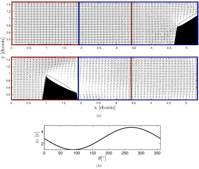
This composite field of view measures the flow over the leading edge of the airfoil throughout its cycle. This suggests that there is some delay caused by the deceleration of the airfoil in the combined pitch/surge motion.

Background
Vertical axis wind turbines
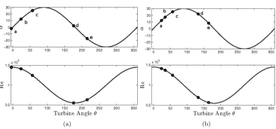
Lift-based turbines provide torque to turn the turbine over the entire rotation cycle due to the projection of the lift vector in the direction of turbine rotation. However, it has been shown that due to the significant decrease in free stream velocity in the downstream half of the turbine (180◦ < θ <360◦) due to the upstream blades and turbine structure, significant torque is only produced. in the upstream half of the cycle (0◦ < θ < 180◦) (Islam et al., 2007).

Dynamic stall
- Dynamic stall on VAWTs
This lift deficit remained for a significant portion of the airfoil movement cycle (Rival et al., 2009; Panda and Zaman, 1994). In further work, Prangemeier et al. (2010) tested different pitch motions at the end of a dive motion to mitigate the effect of the TEV trailing edge vortex.
Leading edge vortex and lift force on accelerating bodies
Greenblatt et al. (2013) were able to increase VAWT power by 10% by using feed-forward control with plasma discharge actuators to reduce the size of the dynamic stall vortex; however, they were unable to completely eliminate the vortex.
Vortex formation
Greenblatt et al.(2013) were able to increase VAWT power output by 10% using feedforward control with plasma discharge actuators to reduce the size of the dynamic stall vortex; however, they were unable to completely eliminate the vortex. diameter) and showed that vortex formation time remained consistent with the optimal formation time ˆT ≈4. Regarding the pitching and dipping of flat plates, Baik et al. 2012) showed that for k ≤ 0.5 the LEV circulation increased linearly up to and including vortex separation, which corresponds to this optimal formation time, while atk >0.5 the vortex was pinched off prematurely due to the reversal of the airfoil motion.
Vortex shedding
Rival et al. (2009) also found, in experiments measuring different pitching motions at k = 0.2−0.33, that vortex formation at the leading edge agrees with this optimal time of vortex formation, and suggested that if it were possible change the stroke motion so that a LEV saturated at the peak of the motion could most effectively use the unsteady lift due to LEV formation and dynamic stall. The vortices detach from the airfoil at the current, time-varying trailing edge position and then convect with the free stream, resulting in a vortex street with a periodic traveling path.
Scope
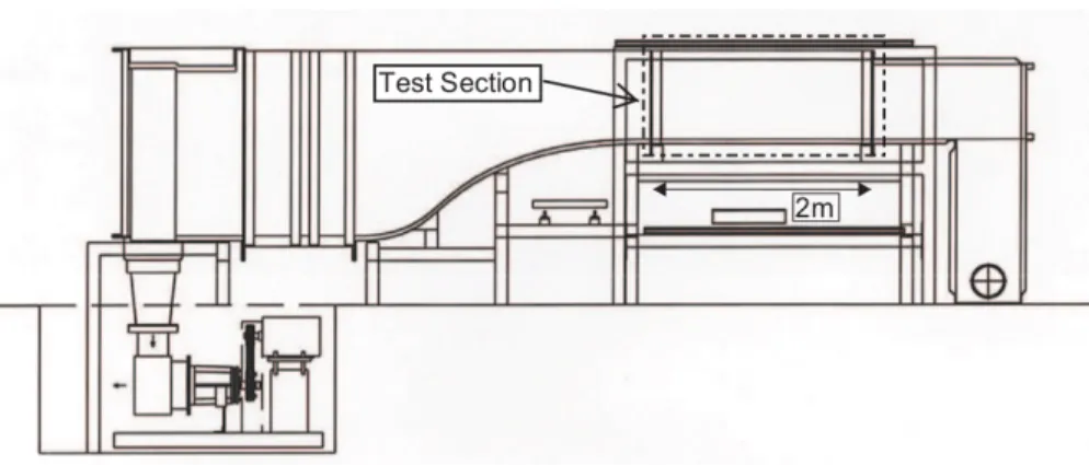
- Test facility
- Airfoil
- Pitch and surge apparatus
- Experimental conditions
The motion frequency in the linear frame, i.e. pitch and pitch frequency, of Ω = 0.6rad s−1 was chosen based on the reduced frequency of the full turbine. Thus, the full-scale conditions of a real VAWT were closely replicated in the linear frame with the notable exception of the Rossby number.
Diagnostics
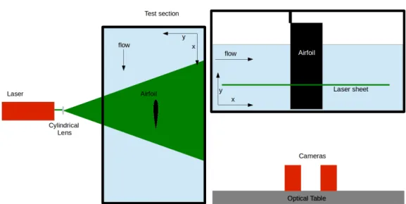
Particle image velocimetry system and setup
Cameras were placed on the side of the test piece with similar overlap downstream of the x/y measurements, providing an approximately 500 mm by 225 mm (2.5×1.13c) field of view in the flow/space direction. It is clear from the schematic (figure 2.6) that the cameras are aligned above the laser head and the laser passes through the bottom of the test section parallel to the airfoil.
Data sets
- Pitch/surge combined motion
- Phase-averaged data
- Instantaneous data
- Pitch motion
- Surge motion
- Reference frame
Due to the lack of jerky motion, experiments were performed only in the front field of view, which was centered below the leading edge of the profile (axis of rotation for pitch). The centrifugal term, however, only appears in the pressure equation as a pressure gradient perpendicular to the airfoil chord.
Analysis techniques
Vortex identification
Tsai and Colonius, 2014), where pis is the pressure, ˆu and ˆx are the velocity and position vectors, respectively, in the rotating frame. Taking the curl and divergence of this equation results in the equations of vorticity and pressure.
Dynamic mode decomposition
The dynamic mode behavior at twice the pitch/voltage frequency is shown in Figure 3.12. A low-order model of the flow across the leading edge was constructed using dynamic mode decomposition.
Three-dimensional effects
Basic velocity profiles
This indicates a separation bubble on the airfoil extending away, iny, from the leading edge into the measurement domain. This separation bubble starts near the leading edge, and the flow reattachs near the center chord;.
Spanwise variation of u
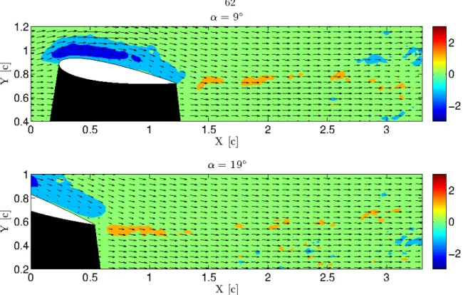
At α=10◦ dieu velocity increases in the region just behind the leading edge, reaches a peak at x/c ~12%, and then drops to close to the free stream velocity behind the airfoil x/c ≥1. This effect is caused by the local acceleration of the flow as it bends around the leading edge of the airfoil.

Mean spanwise flow
Instantaneous measurements
Effect of aspect ratio
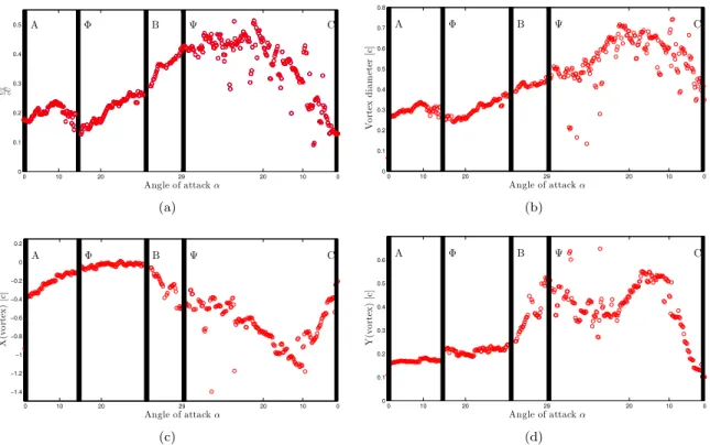
At zero angle of attack, point A (lower right in the figure), the flow is attached to the airfoil, indicated by the vorticity contour following the airfoil surface. From C to A' the airfoil is at negative angle of attack and, as such, the pressure side of the airfoil is visible and the vorticity indicates shear due to the no-slip condition on the airfoil surface.

Low-order model from dynamic mode decomposition
Leading edge vortex circulation
To quantitatively compare the five-mode model with the full flow, the development of the leading edge vortex was analyzed. It is clear that the five-mode DMD model does a very good job of replicating the LEV circulation, capturing both shape and size.
Modal breakdown
Downslope, the oppositely signed vortex appears at α−∼5◦ and slows the reattachment, convecting downstream on the pressure side of the airfoil. The phase relationship also explains the different behavior on the pressure and suction side of the airfoil.
Summary and conclusions
On the suction side of the airfoil (α >0◦ ), the modes act constructively, resulting in separation and subsequent reassembly. The second fundamental time scale investigated is related to the formation growth and shedding of the leading edge vortex.
Timescale II: Leading edge vortex formation
- Attached flow regime
- Leading edge vortex development
- Leading edge vortex separation
- Stalled flow
- Non-phase averaged results
- Vortex formation time
At α∼15◦, point Φ, the leading edge vortex begins to dominate the rotation of the flow around the airfoil and is identified by the Γ criteria. The evolution of the leading edge vortex can be further studied by considering the variation of the vortex circulation with time.
Timescale III: Periodic vortex shedding
This dichotomy between the strength of positive and negative vortices is likely caused by the increased counterclockwise shear imposed on the flow by the downward motion of the airfoil trailing edge during the upslope. Before pointχ and after point B, the vortex content in this frequency band can be seen to extend much further from the airfoil in the y direction and is not only located at the trailing edge position.
Discussion
The vortex deflector at the trailing edge has been rotated to align with the airfoil for clarity. As the leading edge vortex develops and grows toward the trailing edge (Figure 4.20(b)), trailing edge shedding is disrupted.
Summary and Conclusions
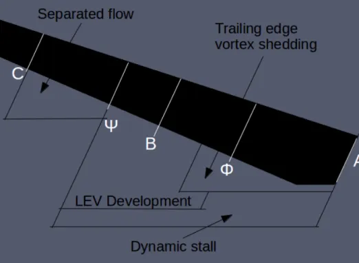
Leading edge vortex development
In this regime, in the pitch-only case, the LEV increases in strength at a constant rate corresponding to the vorticity regime of the pitch/surge flow (Chapter 4). LEV in the pitch-only case begins to grow significantly, bringing more vorticity outside the circular core of the vortex (Figure 5.3(b)).

Vortex formation time
This shares a structure similar to the LEV in the pitch/surge flow during vorticity and corresponds to an increase in the rise rate of the pitch-only LEV circulation. Under this regime, the growth of LEV is faster in the pitch-only case, resulting in a stronger LEV when it falls somewhat before point B (where the pitch/surge LEV falls figure 5.2(b)).
Low-order model of the flow over a pitching airfoil
Modal breakdown
The first mode pair at the peak frequency Ω is shown at separate points in the pitch rise/fall period in Figure 5.10. The phase relationship between the first two mode pairs shown in Figure 5.13 is similar to that of the combined step/over case.

Flow over surging airfoils
Furthermore, unlike the case α= 20◦ , the flow field is dictated by the direction of the airfoil movement. At some point when the airfoil starts to move forward, the opposite happens and the separation point moves forward.
Summary and conclusions
To explore the flow field variation between high Reynolds number experimental data (EPME) and the lower Reynolds number calculations by Tsai and Colonius (2014) in both reference frames (EPME and VAWTC), the vorticity in the laboratory frame at different phases of airfoil motion is plotted in Figure 6.1- 6.4. Finally, the reconnection and fully separated flow appear in the last third of the upstream half of the turbine cycle (120◦≤θ <180◦).
Summary
In the dynamic stall development regime (green in Figure 6.6) the airfoil is initially at zero angle of attack, with rotational speed slowing to a near stop when the flow stops completely before maximum α. From this projection it is clear that while the unsteady effects of LEV surge and shedding are evident on any blade, that blade is the only one in the upper half of the turbine as in Figure 6.7(b).

Opportunities for VAWT design
Direct comparison of the flow field relative to the airfoil showed that the mean flow field developed very similarly between the experiment (EPME) and the computational results in both the equivalent pitch motion/elevation motion of the glider (EPMC) and in the turbine frame (VAWTC) upstream. division. Furthermore, the flow was found to be in good qualitative agreement with the calculations of Tsai and Colonius (2014), indicating the validity of the height/rise approximation.
Future work
Analysis of the pitch and wave motion independently showed that the wave motion added a phase delay to the dynamic stall modes, delaying separation on the airfoil. Simulation of dynamic stall in a two-dimensional vertical axis wind turbine: verification and validation with particle image velocity data.
Top view schematic of typical drag based VAWT (left). Clockwise rotation is driven by
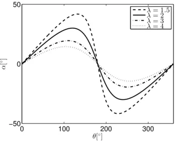
Top view of a typical VAWT. Wind speed U ∞ , relative velocity U , blade velocity ωR,
CAD model of the pitch/surge mechanism
Picture of pitch/surge apparatus installed in test section
Schematic of PIV setup for streamwise/cross-stream measurements
Schematic of PIV setup for streamwise/spanwise measurements
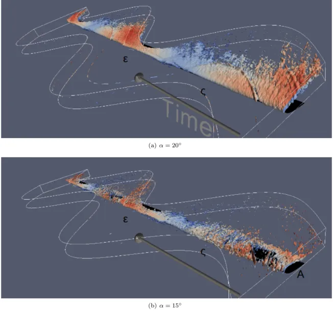
Field of view in the airfoil-fixed frame. Time is extruded in the z direction to show