Indonesia's low infrastructure rating has been a significant obstacle to the realization of robust and sustainable economic growth as well as economic competitiveness in the country. In the medium term, however, public investments in infrastructure will affect production from the supply side through increased economic capacity. DSGE model for analyzing the impact of public spending on the economy One of the models used to analyze the impact of structural reforms in terms of public spending is the DSGE model.
Ganelli and Tervala's paper indicated that government investment increased output in the medium term. In the case of Indonesia, studies on the impact of government spending on output have been conducted by Jha et al. The results show that fiscal policy in the form of lower taxes can have a beneficial effect on the five ASEAN members.
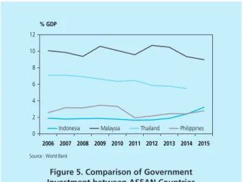
In addition, the impact of monetary policy is more pronounced than that of banking policy in the form of risk-weighted assets (RWA). An increase in the reserve calculated on the basis of the ratio of changes in national income to changes in government spending or tax revenue. Despite recent improvements, several aspects of Indonesia's infrastructure lag behind peers in the region.
Compared to peer countries in the region, Indonesia remains below Malaysia and Thailand in terms of all LPI aspects, namely customs, infrastructure, international shipping, logistics skills, tracking and recording as well as timeliness.
DSGE MODEL
- Households
- Firms
- Fiscal and Monetary Policy 1. Fiscal Policy
- Trade Balance
- Measuring the Output Multiplier and Welfare Multiplier of Government Spending
- Optimal Solution of the Model
- Steady State Value
- Parameterization
2 where β is discount factor, σ is intertemporal elasticity of household replacement, φ is labor supply elasticity, and ν is weight of public consumption. Meanwhile, the log-linear form of the consumer price index equation (5) in a steady state produced 𝑝𝑡= (1 − 𝛼)𝑝𝐻,𝑡+ 𝛼𝑝𝐹,𝑡, so 𝑝𝑛 ,𝑡 = 𝑝 𝑡. Thus, a change in the Consumer Price Index (CPI) is determined by a change in domestic prices and a change in the terms of trade (ToT).
The value of is called the price premium and is determined by the elasticity of substitution between domestic products 𝜀. 12 Equation (12) shows that a change in the optimal price at time 𝑡 (𝜋𝑡) is the weighted average of the marginal costs in the current period and future price changes. The balance of trade, represented by 𝑛𝑥𝑡, illustrates the net exports of domestic production as a ratio of the stable production 𝑌̅.
To measure the impact of public spending on welfare, the present value of the impact of fiscal expansion (𝜏𝑡) on welfare is measured as the portion of consumption households are willing to release due to fiscal expansion. 17 In addition, the output multiplier can also be measured from the present value of the fiscal multiplier (NPVFM), which is calculated as the ratio between the present value of the change in output and the present value of the change in the public sector. expenses in a given period. Therefore, the welfare multiplier effect is obtained from the cumulative change in utility (multiplied by the discount factor) and divided by the cumulative public consumption.
Based on the capital depreciation equation, the value of state intervention in the steady state is equal to the depreciation rate ̅𝐺̅𝑡̅𝐼= 𝜆. The elasticity of substitution between domestic and international goods (𝜂) is assumed to be 3.5, which is consistent with the findings of Obstfeld and Rogoff (1998). Meanwhile, the elasticity of substitution between international goods 𝛾 is assumed equal to 1, according to Gali and Monacelli (2005).
The elasticity of substitution of labor supply as 𝜑 is assumed at 1.97, which is the same as Sin (2016) and not much different from Ganelli and Tervala (2015). The value of the Calvo parameter 𝜃 = 0.5 is assumed at 0.5, a value often used in many New Keynesian models and the same as Tjahjono et al. 2009) for the Indonesian Structural Macromodel (BISMA). Public infrastructure is assumed to depreciate every quarter at a rate of 𝜆 = 0.025, which is the same as the depreciation rate used in the Bom and Ligthart (2014) model.
The output elasticity of public infrastructure stock, 𝜙𝑘, is a key parameter in this paper, with 𝜙𝑘 = 0.24, in line with the results of Aschauer (2000) for the case of low- and middle-income countries. More details, the prior distribution, distribution type and posterior distribution of the parameter estimates are presented in Table 5.
Simulation Results
Government Consumption
On the one hand, higher taxes would lead to lower household consumption and then a benefit, while working hours would have to be increased to compensate for the additional costs. On the other hand, government consumption as part of utility directly increases welfare. The simulations also show that the welfare multiplier of increased government consumption had a value of -0.001, meaning that households would have to sacrifice Rp0.001 of consumption for every Rp1 the government spent on consumption.
The results are consistent with the findings of Ganelli and Tervala (2015), in which increased government consumption reduces household welfare. Nevertheless, the model can also result in a positive welfare multiplier if the ratio of government consumption spending to household consumption (parameter) ≥0.2, implying that the minimum ratio of government consumption is 20% of household consumption to neutralize the adverse effect of increased government consumption .
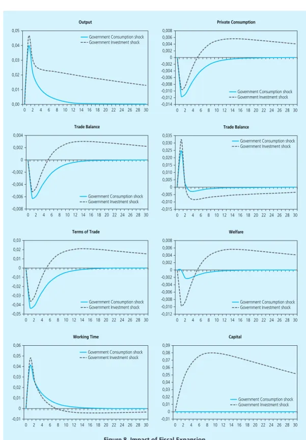
Government Investment
As shown in Figure 8, consumption will fall in the short run, dampened by an increase in taxes to offset government investment spending. Moreover, higher investment spending would improve the terms of trade (ToT), thereby strengthening purchasing power and consumption growth, although still negative in aggregate due to the dominant effect of higher taxes. Although consumption would fall, large-scale investment would push the trade balance into a deficit.
Nevertheless, in the long run, consumption and the trade balance would strengthen as industry became more productive. These findings are consistent with Iwata (2013) who found that a government investment shock would worsen the trade balance in the short run but then improve in the medium run. The simulations also show that the welfare impact of government investment is 0.05, meaning that households receive a net benefit of Rp 0.05 for every additional Rp1 of government investment.
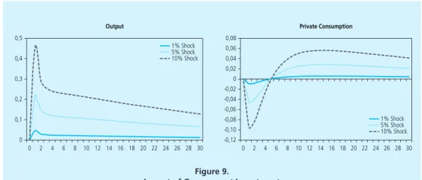
The net gain is an increase in consumption due to greater productivity without having to increase working hours. A higher investment value would lead to a more significant increase in production in the short term as well as in the medium term. The impact on other macro conditions such as consumption, balance of trade, inflation and welfare also results in similar results.
Bom and Ligthart (2014) show that the impact on welfare is sensitive to changes in the output elasticity of public capital. Using the same analysis, this study shows that as the new public infrastructure became more productive, the potential increase in economic growth and impact on welfare would also increase (Table 7). Such dynamics indicate that priority infrastructure development should focus on improving productivity to provide the most optimal benefits to the economy.
Conclusions
