Our findings may be due to the timing of the panel, as it took place precisely during macroeconomic turmoil resulting from a severe financial crisis. Second, high inequality can be attributed to the unstable labor markets and macroeconomic performance of the region. However, this geographical bias does not seem to affect the other characteristics of the data.
If it is assumed that these two terms are uncorrelated and the latter are independently and identically distributed across periods and individuals, then the variance of the dependent variable can be additively decomposed into the variance of the permanent component plus the variance of the temporary component. The neat decomposition of the variance of earnings allows us to determine what part of the total inequality (as measured by the variance of the logarithmic earnings) is explained by the inequality in the permanent component. The general structure implied by equations (4) to (6) assumes a fixed earnings growth profile and a fixed variance of the permanent component over time and across individuals.
Lillard and Weiss (1979) and, more recently, Baker (1997) and Baker and Solon (1999) introduce a much more complex permanent component, which allows the variance of the permanent component to vary depending on individual specific work experience profiles.6. Given the data availability and the characteristics of the variance-covariance structure of Venezuelan data described in the previous section, we start with one. Unlike other variance component decomposition studies, our data are collected twice a year. that the initial conditions for the variance of the .. transient component are stable. so 1 2.
This allows us to measure how much of the permanent and transitory components are explained by characteristics associated with human capital formation and other observables associated with labor market outcomes.
Estimation Results
A decomposition of hourly wages
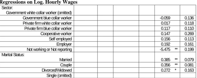
We create a panel of men in the same age group, but who work no less than thirty hours a week during the five semesters under study. Hourly wages are calculated by dividing monthly earnings by hours worked during the previous month (which is calculated as 4.3 times the weekly hours answered to the question “How many hours did you work last week?”) This subsample of only 656 observations has much less variation in number of hours worked than the previous sample and therefore most of the variation in the dependent variable should not be greatly affected by changes in hours worked. Compared to Table 2, we notice that this data set is similar to the previous one we used.
Income and mean age and education, as well as the distribution by occupation, industry, region, and marital status, are nearly identical across samples. Surprisingly, we find a similar distribution of wage variance in permanent and transitory components. One important difference, however, is that the coefficient for serial correlation is no longer significant.
This suggests that differences in hours worked are the source of the serial correlation structure for the transitory component in monthly earnings. This means that changes in working hours have some permanent effect on earnings over time, albeit a small one. It is interesting that the transitory component is so dominant, even if we focus on always employed people.
First, inflationary shocks that suddenly change real wages can cause a lot of variability if workers cannot, as they usually do not, fully index their wages. Second, a recession not only affects the number of people employed by reducing the labor force, but also causes equilibrium real wages to fall, unless there is a commensurate change in the supply of labor. Third, in a dual labor market, individuals may continue to work in all periods but move to a less productive sector where they work longer hours for a lower age to maintain the same earnings.
All these three cases cause instability of real hourly wages, which is consistent with our findings of a large transitory component in the variance of hourly wages.
Summary and Conclusions
After fitting several models, we find that the permanent component accounts for about 22% of earnings inequality as measured by the variance of logarithmic real monthly earnings, while the stochastic component accounts for 77% and the remaining 1% corresponds to serial correlation. This contrasts with the findings of the error components literature for developed countries where the permanent component is found to be larger or at least as large as the transient component, for example Baker and Solon (1999), Dickens (1996), Gottschalk and Moffitt (1995). This large transitory component may be a consequence of the instability that characterizes the Venezuelan economy during this period.
On the one hand, this implies that there is a high degree of income mobility among prime-age Venezuelan men, and that therefore the high inequality measured on the basis of cross-sectional data for this country does not necessarily equal high inequality in the long run entails. On the other hand, this large temporary component also implies that lower levels of inequality could be achieved in the short run if the economy had a more stable labor market. Holtz-Eakin and S.Rhody (1997) “Labor Earnings Mobility and Inequality in the United States and Germany during the growth years of the 1980s”, International Economic Review, vol.38, no.4, pp. The evolution of individual male earnings in Britain Center for Economic Performance Discussion paper n.
Lemieux, “Divergent Wage Inequality among Men in the United States and Canada Can Institutions Explain the Difference?” Industrial and Labor Relations Review, July 1997, 50, pp.629-651. Freije, Samuel (2001) “Mobility and distribution of household income during macroeconomic instability in Venezuela” in Household Income Dynamics in Venezuela, unpublished Ph.D. Autor (1999), “Changes in Wage Structure and Income Inequality,” in Handbook of Labor Economics, Volume 3-A, ed.
1982), "Using Time Series Processes to Model the Error Structure of Earnings in an Analysis of Longitudinal Data". Journal of Econometrics 18, pp The Covariance Structure of Earnings in British Great Institute for Social and Economic Research, working paper 99-4, University of Essex. 1995) “The Changing Structure of Male Earnings in Britain in Differences and Changes in Wage Structures, ed. Monthly earnings for men aged 25 to 55, after controlling for panel wave, age, education and migration.
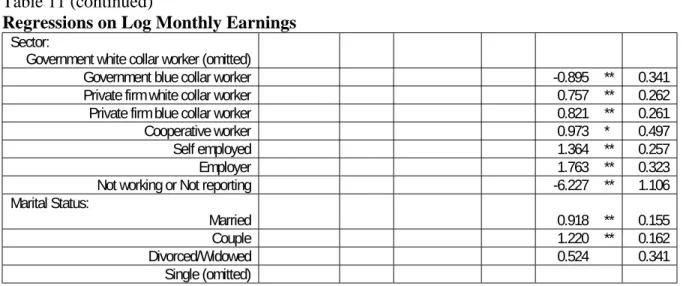
Monthly income of men aged 25 to 55 after controlling for panel wave, age, schooling, migration and labor market characteristics (2). First we include only panel wave dummies, then we add a quartic of age, education and migration status, and in the third stage we add occupation, industry, region, function and marital status. With these residuals, we calculate a sample autocovariance matrix of dimension TxT, where T is the number of panel waves (in our case 5).
On the other hand, from equations 9 and 10 in the text, we define a column vector g( ), with the same dimension as , which consists of a series of linear or nonlinear constraints on the vector of parameters.