Eigenvalue Inequalities in Quantum Information Processing

(1)

Processing

Thesis by

Sumit Kumar Daftuar

In Partial Fulfillment of the Requirements for the Degree of

Doctor of Philosophy

California Institute of Technology Pasadena, California

2004

(Defended September 25, 2003)

(2)

c 2004

(3)

Acknowledgements

Many people have helped me in this endeavor.

My advisor, John Preskill, was gracious enough to accept me as a mathematics student into his research group. His wonderful course on quantum information theory introduced me to the subject. He also provided guidance on problems to consider answering, and where to look for help in solving them, on various occasions.

Michael Nielsen introduced me to the subject of majorization and its applications to quantum information theory. He suggested a lot of useful questions which got me started on the problem considered in Part I of this thesis. He also provided helpful encouragement and feedback on some of the work in Part I. In addition, he taught me some representation theory.

I collaborated with Matthew Klimesh on some of the work presented in Part I of this thesis (essentially, the last three sections of Chapter 2).

Patrick Hayden was my collaborator on Part II of this thesis. Perhaps “mentor”

would be a better word to describe his role. He introduced me to the problem and recognized how to generalize my initial line of attack; from that point, he guided our joint efforts. Along the way, he explained many difficult concepts to me. In the context of all this, it seems hardly worth mentioning that he also provided extensive comments on a draft of this thesis and drew one of the figures for me. I cannot thank him enough.

Michael Hartl helped me learn L^ATEX, and more recently, helped me with thesis- specific L^ATEXissues. Long before that, he was my study partner in virtually every undergraduate physics course I took (and some math courses too), and has undoubt- edly influenced my thinking in ways I don’t even realize.

(4)

I also wish to thank Charlene Ahn, Michael Aschbacher, David Bacon, David Beckman, John Cortese, Christopher Fuchs, Jim Harrington, Rowan Killip, Allen Knutson, Andrew Landahl, Debbie Leung, Carlos Mochon, Benjamin Rahn, Eric Rains, Guifr´e Vidal, Clint White, and Richard Wilson, whose helpful discussions (in some cases, courses) enhanced my understanding of physics and/or mathematics during my time at Caltech.

(5)

Abstract

This thesis develops restrictions governing how a quantum system, jointly held by two parties, can be altered by the local actions of those parties, under assumptions about how they may communicate. These restrictions are expressed as constraints involving the eigenvalues of the density matrix of one of the parties. The thesis is divided into two parts.

Part I (Chapters 1–4) explores what is possible if the two parties may use only classical communication. A well-known result by M. Nielsen says that this is intimately connected to themajorizationrelation: if xis the vector of eigenvalues of the initial state, thenycan be the vector of eigenvalues of the final state if and only ifxis majorized byy. It was recently observed that it is possible forx⊗z to be majorized byy⊗z, even ifx is not majorized by y; physically, this means that the presence of a state with eigenvalues z is a catalyst that allows a certain transformation to occur.

If such a z exists, then x is said to be trumped by y. Part I is mainly a study of the structure of this trumping relation, an extension of the majorization relation.

Notably, we show that for almost all probability vectors y ∈ R^d where d ≥ 4, there is no finite dimensionn such that the set of vectors trumped by y can be determined by restricting attention to catalysts of dimension n. We also study some concrete examples to illustrate various aspects of the trumping relation.

Part II (Chapters 5–9) considers the question of how a state can change as a result of quantum communication between the parties; i.e., one party sends the other a portion of the jointly held quantum system. Given the spectrum of the initial state, it turns out that the possible spectra of the final state are given by the solutions to linear inequalities. We develop a method for deriving these inequalities, using a

(6)

variational principle. In order to apply this principle, we need to know when certain subvarieties of a Grassmannian variety intersect, which can be a regarded as a problem in Grassmannian cohomology. We discuss this cohomology and derive the conditions for nontrivial intersection. Finally, we illustrate how these intersections give rise to the desired inequalities.

(7)

List of Figures

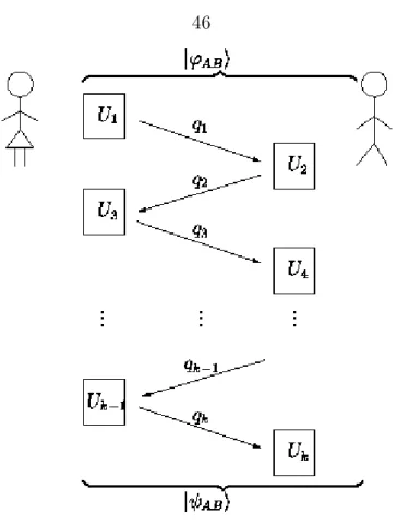
5.1 A many-round quantum communication protocol . . . 46 9.1 Partitions, their Schur polynomials and binary strings . . . 93

(11)

Part I

Mathematical Structure of Entanglement

Catalysis

(12)

Chapter 1

Majorization

We begin by introducing the theory of majorization, a mathematical relation that has recently been shown to have striking applications to quantum information theory. Majorization constraints have been shown to govern transformations of quantum entanglement [1], to restrict the spectra of separable quantum states [2], and to characterize how quantum states change as a result of mixing or measurement [3]. It has even been suggested that all efficient quantum algorithms must respect a majorization principle [4]. Our purposes will be to introduce some background facts that will be useful to us, and to demonstrate various ways of characterizing the majorization condition. Because our main goal for Part I will be to study an extension of the majorization relation (known as trumping), such characterizations will serve as an illustration of the types of results we seek for the trumping relation. This chapter consists of background material that can be found in a reference such as [5] or [6].

1.1 Definition and Motivation

Let x = (x1, . . . , xd) and y = (y1, . . . , yd) ∈ R^d. We will be most interested in the case where x and y are are d-dimensional probability vectors; in other words, their components are nonnegative and sum to unity. However, for most results in the theory of majorization, this restriction is not needed. Letx^↓ denote thed-dimensional vector obtained by arranging the components ofxin non-increasing order: x^↓ = (x^↓₁, . . . , x^↓_d), where x^↓₁ ≥ x^↓₂ ≥ · · · ≥ x^↓_d. Then we say that x is majorized by y, written x ≺ y, if

(13)

the following relations hold:

`

X

i=1

x^↓_i ≤

`

X

i=1

y_i^↓ (1≤` < d) (1.1)

and

d

X

i=1

x^↓_i =

d

X

i=1

y_i^↓. (1.2)

Intuitively, ifxand y are probability vectors such thatx≺y, then xdescribes an unambiguously more random distribution than does y. For example, in R², we have that (0.5,0.5)≺(0.8,0.2). In fact, (0.5,0.5) is majorized by every vector in R² whose components sum to unity.

The majorization relation defines a partial order on d-dimensional real vectors, where x ≺ y and y ≺ x if and only if x^↓ = y^↓. To see that majorization is not a complete relation, consider for instance x = (0.5,0.25,0.25) and y = (0.4,0.4,0.2);

then x6≺y and y6≺x.

Majorization was introduced to formalize the notion of what it means for one vector to be unambiguously less disordered (or alternatively, more unequal) than another. Some of the beginnings of the theory originate from economics, where it played a role in comparing income and wealth distributions. We will illustrate the meaning of majorization in terms of this idea, to motivate the definition given by Inequalities 1.1 and Equation 1.2. Consider two populations X and Y, each of d individuals. Let xi be the wealth of individual i in population X, and let yi be the wealth of individual i in populationY. Suppose for simplicity that the total amount of wealth in the two populations is the same, P

ixi = P

iyi (we can divide each term x_i and y_i byP

ix_i and P

iy_i, respectively, to normalize for differences in total wealth). Now, suppose that the richest individual in population Y has at least as much wealth as the richest individual in populationX, the two richest individuals in population Y have at least as much combined wealth as the two richest individuals in population X, etc. (Note that because the total amount of wealth is equal in the two populations, this is equivalent to saying that the poorest individual in population

(14)

X has at least as much wealth as the poorest individual in population Y, the two poorest individuals in X have at least as much combined wealth as the two poorest individuals in Y, etc.) Then it is reasonable to say that (x₁, . . . , x_n) represents a more equal distribution of wealth than (y₁, . . . , y_n). This notion of inequality was introduced by M. O. Lorenz [7] in 1905. In our notation, this is saying precisely that

`

X

i=1

x^↓_i ≤

`

X

i=1

y_i^↓, (1.3)

i.e., that x is majorized by y.

Another way of evaluating wealth inequality is by considering the effects of transfers of wealth. Letiandj be two individuals in a populationX, where without loss of generality we assume thatx_i ≤x_j. A transfer of wealth is said to take place ifj (the wealthier member) gives some wealth to i, but not so much that i is now wealthier than j used to be. Mathematically, (x_i, x_j) gets mapped to the convex combinations (tx_i+ (1−t)x_j,(1−t)x_i+tx_j), for somet ∈[0,1]. The effect of a transfer is to make the overall wealth distribution more equal; this suggests that we define one wealth distribution to be more equal than another, if it can be obtained from the other by a series of wealth transfers. This notion of inequality was suggested by E. C. Pigou [8] and H. Dalton [9] in the early 20th century. It turns out that these two notions of inequality are equivalent, a fact which we will prove in the next section.

1.2 T -transforms

Define a linear mapT fromR^d to R^d to be a T-transformif there exist t∈[0,1] and indices j, k such that

T(y) = (y₁, . . . , y_j−1, ty_j + (1−t)y_k, y_j+1, . . . ,(1−t)y_j +ty_k, y_k+1, . . . , y_d).

Then we have the following theorem:

Theorem 1.2.1 Let x and y be vectors in R^d. Then x ≺ y if and only if x can be

(15)

obtained from y by a finite number of T-transforms.

Proof It is easy to see that T(y)≺y for any T-transform T, so if D=T₁. . . T_r is a product ofT-transforms, then x=D(y)≺y. This proves one direction.

For the other direction, we will use induction on d, the dimension of the vector space of whichxandy are elements. Clearly, the result holds for the base cased= 2.

Suppose the statement is true for a given dimensiond, and thatx≺y for vectors x, y ∈ R^d+1. We may assume without loss of generality that x = x^↓ and y = y^↓. Since x≺y,y_d+1 ≤x_d+1 ≤x₁ ≤y₁, so there must be a k ∈ {1, . . . , d+ 1} such that y_k≤x₁ ≤y_k−1. So there existst∈[0,1] such thatx₁ =ty₁+ (1−t)y_k. Let T be the T-transform that mapsy₁ toty₁+ (1−t)y_k, and maps y_k toty_k+ (1−t)y₁):

T y = (ty₁+ (1−t)y_k, y₂, . . . , y_k−1,(1−t)y₁ +ty_k, y_k+1, y_d+1) (1.4)

= (x₁, y⁰), (1.5)

where

y⁰ = (y2, . . . , yk−1,(1−t)y1+tyk, yk+1, yd+1). (1.6) Define x⁰ = (x₂, x₃, . . . x_d+1). Now x⁰ and y⁰ are d-dimesional vectors, so we will show that x⁰ ≺ y⁰ in order to apply the inductive hypothesis. Suppose first that 1≤`≤k−2. Then since y_k−1 ≥x₁, we have that

`

X

j=1

x⁰_j =

`+1

X

j=2

xj (1.7)

≤

`+1

X

j=2

y_j (1.8)

=

`

X

j=1

y⁰_j (1.9)

≤

`

X

j=1

(y⁰_j)^↓. (1.10)

(16)

Next suppose that k−1≤` ≤d. Then we have

`

X

j=1

(y_j⁰)^↓ ≥

`

X

j=1

y_j⁰ (1.11)

=

k−1

X

j=2

yj + [(1−t)y1+tyk] +

`+1

X

j=k+1

yj (1.12)

=

`+1

X

j=1

y_j −[ty₁+ (1−t)y_k] (1.13)

=

`+1

X

j=1

y_j −x₁ (1.14)

≥

`+1

X

j=1

x_j −x₁ (1.15)

=

`+1

X

j=2

x_j (1.16)

=

`

X

j=1

x⁰_j. (1.17)

We have thus shown that x⁰ ≺ y⁰. Therefore, there is a sequence T₁, . . . T_r of T- transforms on R^d such that x⁰ = T₁· · ·T_ry⁰. But we may regard each T_i as a transformation on R^d+1 that fixes the first coordinate, so we have that x = T₁. . . T_rT y.

2

Corollary 1.2.2 The two notions of wealth inequality given in the previous section are equivalent.

1.3 Geometric Characterization

Recall that a d×d matrix A is said to be doubly stochastic if all of its entries are nonnegative, and each row and column ofA sums to unity. For instance, is not hard to see that every T-transformation is a doubly stochastic map, and that products of doubly stochastic maps are doubly stochastic. The study of doubly stochastic matrices is well-known to be connected to the theory of majorization [10, 11]:

(17)

Theorem 1.3.1 (a) Ad×dreal matrixAis doubly stochastic if and only if Ay≺y for all y∈R^d.

(b) x≺y if and only if there is a doubly stochastic matrix A such that x=Ay.

If we think of x and y as probability vectors, then Theorem 1.3.1 (a) tells us that the doubly stochastic matrices are precisely those matrices that map any probability distribution to one that is at least as mixed.

Given a vector y ∈ R^d, define S(y) to be the set of vectors x ∈ R^d such that x ≺ y. By Theorem 1.3.1, S(y) = {Ay|A is doubly stochastic}. In this section we will establish Birkhoff ’s theorem, which gives a geometric description of the doubly stochastic matrices, and use it to give a geometric description ofS(y).

We begin with themarriage problemfrom combinatorics [12]. LetB andGbe two finite sets of the same cardinality, and let R be a relation on B×G. We think of the elements of B and G as “boys” and “girls,” respectively, and R(b, g) as the relation that b ∈ B and g ∈G love one another. A compatible matching is a pairing of each boy with one girl (distinct for each boy) such that only couples who love one another are paired up. The marriage problem is to determine when a compatible matching exists, given B×G and R. The solution is given by Hall’s theorem:

Theorem 1.3.2 (Hall’s Theorem) A compatible matching forB×G andR exists if and only if every group of k boys loves at least k girls, for k ∈ {1, . . . ,|B|}.

Proof Clearly, if a compatible matching exists, each group of k boys loves at least k girls (those girls chosen to be their matches).

For the reverse direction, we proceed by induction. The base case |B|= 1 is clear, so assume the statement is true when |B| ≤n; we wish to prove it for |B|=n+ 1.

Suppose first that there existsk ∈ {1, . . . , n}such that there is a groupβofkboys who love a group γ of exactly k girls. Then β and γ can be compatibly matched, by the inductive hypothesis. The complements β^c and γ^c can also be compatibly matched: if S is a subset of β^c containing h members, then by assumption, the set β∪S of k+h boys loves at least k+h girls, so that the h boys of S must love at

(18)

least h girls in γ^c. This implies that β^c and γ^c can be compatibly matched, by the inductive hypothesis.

Now suppose that the assumption of the previous paragraph is false, meaning that for eachk ≤n, all groups ofk boys love at leastk+ 1 girls. In this case we can simply take one boy and girl who love each other, and pair them together. The remaining n boys and n girls now satisfy the inductive hypothesis. 2 Hall’s theorem is equivalent to the following theorem on matrices. Given a d×d matrix A, define a diagonal of A to be a set {a_1π(1), a_2π(2), . . . , a_dπ(d)}, where π is a permutation of{1, . . . , d}.

Corollary 1.3.3 (K¨onig-Frobenius Theorem) A d×d matrix A contains a diagonal with no zero elements if and only if every k×l zero submatrix of A satisfies k+l ≤d.

Proof We construct a marriage problem from the matrix A. The boys correspond to the rows of A, and the girls correspond to the columns; boy i and girl j love one another if and only if A_ij 6= 0. Then a compatible matching occurs if and only if A has a nonzero diagonal. By Hall’s theorem, this happens if and only if each group of k boys loves at leastk girls; i.e., for every k×l zero submatrix, k≤d−l. 2

We are now ready to prove Birkhoff’s theorem.

Theorem 1.3.4 (Birkhoff ’s Theorem) The set ofd×ddoubly stochastic matrices is a convex set whose extreme points are the d×d permutation matrices.

Proof It is straightforward to check that the set ofd×ddoubly stochastic matrices is convex, and that the permutation matrices are extreme points of this set. So we must show that any doubly stochastic stochastic matrixDcan be written as a convex sum of permutation matrices:

D=X

i

p_iP_i. (1.18)

Let n(D) be the number of nonzero matrix elements of D. Because each row must have at least one nonzero entry, n(D)≥d. We use induction onn(D). For the base case n(D) = d, D has only one nonzero entry in each row and in each column, this

(19)

nonzero entry must therefore be 1. It follows that D itself is a permutation matrix, so the statement is true for the base case.

For the inductive step, first note that the sum of all the elements of D must be equal to d. If D has a k ×l submatrix, then the sum of the elements of the k rows corresponding to this submatrix, plus the sum of the elements of the l columns correspond to the submatrix, must be less than the sum of all elements ofD, since no nonzero element is included more than once in the sum. Therefore,k+l ≤d. So we may apply the K¨onig-Frobenius theorem to conclude that there must be a diagonal of D with only nonzero elements. Choose any such diagonal, and let p be the smallest element on this diagonal, and P be the permutation matrix whose ones are on this diagonal. If p= 1, then D must be a permutation matrix, so we are done. Consider the case 0< p <1. Let Q be the matrix defined by

Q= D−pP

1−p . (1.19)

ThenQis doubly stochastic and has fewer nonzero entries thanD, so by the inductive hypothesis, we may write Q as a convex sum of permutation matrices:

Q=X

i

p_iP_i. (1.20)

But D= (1−p)Q+pP, so

D=pP +X

i

(1−p)p_iP_i (1.21)

is a convex sum of permutation matrices. 2

Birkhoff’s Theorem and Theorem 1.3.1 together imply the following:

Theorem 1.3.5 For any y∈R^d, S(y) is a convex set whose extreme points are the elements of the set {P y|P is a d×d permutation matrix}.

(20)

1.4 Schur-convexity

Much of the power of majorization comes from the theory of Schur-convexity, which allows one to derive inequalities from an appropriate majorization condition. A function f : R^d → R is said to be Schur-convex if f(x) ≤ f(y) whenever x ≺ y. If f(x) ≥ f(y) whenever x ≺ y, then f is said to be Schur-concave. While it is not obvious that interesting Schur-convex (or Schur-concave) functions should exist at all, the following theorem shows how to construct many such functions:

Theorem 1.4.1 If I ⊂R is an interval and g :I →R is convex (concave), then the function

φ(x) =

n

X

i=1

g(x_i) is Schur-convex (Schur-concave) on Iⁿ.

Proof In view of Theorem 1.2.1, it is sufficient to show that φ(x) ≤ φ(y) whenever x = T y for some T-transform T. Without loss of generality, suppose T acts non-trivially on the first two components of y, so that x₁ = ty₁ + (1−t)y₂, x₂ = (1−t)y₁+ty₂, and x_i =y_i for i >2. Then g(x₁) +g(x₂) =g(ty₁+ (1−t)y₂) + g((1−t)y₁+ty₂) ≤ tg(y₁) + (1−t)g(y₂) + (1−t)g(y₁) +tg(y₂) = g(y₁) +g(y₂), so

φ(x)≤φ(y). 2

One consequence of Theorem 1.4.1 is the connection between majorization and entropy, a more familiar measure of randomness. Because the function g(p) =

−plogp is concave on the interval [0,1], it follows that the entropy function H(x) =

−P

ix_ilogx_i is a Schur-concave function. That is, ifx≺y (wherexand yare probability vectors) then H(x)≥H(y). This agrees with our intuition that x≺y means that x describes a more random probability distribution than y does. Of course, majorization is a much stronger condition than the entropy criterion for determining relative randomness: there exist probability vectors x and y such that x 6≺ y, yet H(x) ≥H(y). This is not hard to understand, when we consider that majorization is not a complete relation.

(21)

The notion of Schur-convexity has been used to derive inequalities in many branches of mathematics, notably linear algebra, geometry, and statistics. For example, it can be shown that the diagonal entries of a Hermitian matrix are majorized by its eigenvalues (this is an easy consequence of Ky Fan’s Maximum Principle; see Theorem 6.1.1).

Schur himself used this fact to give a proof of Hadamard’s well-known determinant inequality:

Theorem 1.4.2 (Hadamard Determinant Inequality) Let H be a positive defi- nite Hermitian matrix. Then the determinant ofH is less than or equal to the product of the diagonal entries.

Proof Leth= (h11, h22, . . . , hnn) be the vector of diagonal entries ofH, and let λ(H) = (λ₁(H), . . . , λ_n(H)) be the vector of eigenvalues of H. Because the function g(t) = logt is concave, the function φ(x) = Pd

i=1logt is Schur-concave. Since h ≺ λ(H), it follows that Pd

i=1logλ_i(H)≤Pd

i=1logh_ii. This implies that the product of the eigenvalues is less than or equal to the product of the diagonal entries. 2 The majorization relation itself can be defined in terms of Schur-convex functions.

It is not hard to prove the following directly:

Theorem 1.4.3 Let x, y∈R^d. Then x≺y if and only if for all t∈R,

d

X

i=1

|x_i−t| ≤

d

X

i=1

|y_i−t|. (1.22)

Theorem 1.4.3 has limited use because it is easier to check the defining inequalities for majorization than to check that Inequalities 1.22 are satisfied. However, it has theo- retical value because it shows that Schur-convex functions can be used to characterize majorization:

Theorem 1.4.4 Let x, y ∈ R^d. Then x ≺ y if and only if f(x) ≤ f(y) for all Schur-convex functions f :R^d→R.

Proof The function g_t(s) =|s−t| is convex, so that for anyt∈R and x∈R^d, φt(x) =Pd

i=1|xi−t|is Schur-convex. So iff(x)≤f(y) for all Schur-convex functions

(22)

f, then in particular φ_t(x) ≤ φ_t(y) for all t ∈ R, so x ≺ y by Theorem 1.4.3. The reverse direction follows from the definition of Schur-convex function. 2

1.5 Summary

We collect some useful properties of the majorization relation into the following list:

• Given two vectorsxandy, it is easy to determine whether x≺y (the definition can be checked directly, for example).

• We can intepret x ≺ y as saying that x can be obtained from y via a series of simple mixing operations (transfers).

• The geometric structure of majorization is well-behaved; x ≺ y means that x lies in the convex hull of the vectors obtained by permuting the components of y.

• Majorization can also be characterized function-theoretically, in that there is a family of functionsφ_tsuch thatφ_t(x)≤φ_t(y) for allt is necessary and sufficient for x≺y.

We will keep this list in mind in trying to analyze the related notion of trumping, defined in the next chapter.

(23)

Chapter 2

Introduction to Trumping

In this chapter, we introduce an extension of the majorization relation that will be the main focus of our study in Part I. Given probability vectorsxandy, we ask when there exists a probabability vector z such thatx⊗z ≺y⊗z. (It turns out that this situation may occur even if x6≺ y.) This question arises naturally in studying what transformations of quantum entanglement are possible using only local operations and classical communcation. The mathematical notion may be accurately described as “tensor product induced majorization” but we will use the simpler termtrumping, introduced by M. Nielsen [6]. The material in this chapter, and in the first section of the next chapter, was published previously by the author and a collaborator [13].

2.1 Entaglement Catalysis

Quantum entanglement exists when a quantum mechanical system, consisting of various subsystems, cannot be fully described simply by giving a complete local description of all the subsystems. Entanglement seems to play an essential role in numerous remarkable applications of quantum information science, including quantum cryptog- raphy [14, 15], quantum teleportation [16], and superdense coding [17]; because of this, it has come to be viewed as a fundamental resource that allows one to perform certain information-processing tasks. As with any physical resource, one wishes to measure how much entanglement is present in a given system, and to determine under what conditions it is possible to convert one form of entanglement to another. The

(24)

problem of how to quantify and classify entanglement is one of the basic questions in the study of quantum information [18, 19].

The following theorem due to M. Nielsen shows that the structure of bipartite quantum entanglement is intimately related to majorization [1]:

Theorem 2.1.1 Suppose Alice and Bob are in joint possession of a bipartite entangled quantum state |ψi which they wish to transform into another bipartite entangled state |φi using only local operations and classical communication (LOCC). Let |ψi= Pd

i=1

√α_i|i_Ai|i_Bi be a Schmidt decomposition of |ψi, and let |φi=Pd i=1

Nielsen’s theorem defines a partial order on the entangled bipartite pure states.

If state |ψi has x as its vector of Schmidt coefficients, and |φi has y as its vector of Schmidt coefficients, then we can transform |ψi to|φi using LOCC if and only if x ≺ y. Because our ability to transform one state to another depends only on their Schmidt coefficients, and not on the bases, we shall abuse nomenclature and refer to any vector of Schmidt coefficients as a “state.”

Jonathan and Plenio have extended Nielsen’s result by describing a phenomenon known as entanglement catalysis [20]. Suppose that x = (0.4,0.4,0.1,0.1) and y = (0.5,0.25,0.25,0). Then x6≺y. Now letz = (0.6,0.4). Then we have x⊗z ≺y⊗z.

In other words, if Alice and Bob start only with state x(by which we mean a jointly entangled quantum state whose Schmidt coefficients are the components of x), they cannot transform it into statey using LOCC. But if they also have statez available, then they can turnx⊗z intoy⊗z. So they can “borrow”z, use it to help turnxinto y, and “return” it after performing the transformation. We say that z is a catalyst for the transformation.

The phenomenon of catalysis illustrates that entanglement itself can be used as a resource to help perform transformations of entangled states. One naturally wishes to know when this is possible: given x and y, can we determine whether x can be transformed to y using LOCC in the presence of a catalyst? This is equivalent to

(25)

asking whether there is a probability vector z such that x⊗z ≺y⊗z. Transforma- tions using LOCC together with a catalyst are termed entanglement-assisted LOCC transformations, abbreviated asELOCC transformations.

2.2 Definitions and Basic Properties

We will adopt the terminology and notation introduced by Nielsen [6] and say that x is trumped by y, written x ≺T y, if there exists a catalyst z (of any dimension) such that x⊗ z ≺ y ⊗ z. For any given y, let T(y) denote the set of all x such that x is trumped by y; and for any y and z, let T(y, z) be the set of all x such that x ⊗ z ≺ y ⊗ z. In addition, we introduce the following notation: for any d-dimensional probability vector y and any positive integer k, let Tk(y) ={x| ∃ a k-dimensional probability vectorz such that x⊗z ≺y⊗z}.

In contrast to the situation with the majorization relation, the mathematical structure of the trumping relation is not well understood. One desires a necessary and sufficient condition for determining whether x≺T y (or alternately, to determine the elements of the setT(y) for any giveny). Characterizing the trumping relation in this way would help us to better understand the structure of the bipartite entangled states. However, such a characterization is not yet known. Part I of this thesis describes progress made in learning about the structure of this relation.

Our results will rely heavily on the fact that the trumping relation involves vectors with all nonnegative components. Note that this is quite different from the situation with majorization, in which most results extend easily to vectors containing negative components.

The following proposition lists some elementary facts about the trumping relation.

Proposition 2.2.1 Let x andy be d-dimensional probability vectors, let z be a probability vector (of any dimension), and let S(y), T(y), and T_k(y) be defined as above.

Then

(a) x≺y⇒x⊗z ≺y⊗z.

(26)

(b) S(y)⊆T(y).

(c) T(y) =S∞

k=1T_k(y).

(d) If x≺T y, then x^↓₁ ≤y^↓₁ and x^↓_d≥y_d^↓. (e) T(y) is a convex set.

(f ) Ifx≺T y and y≺T x, then x^↓ =y^↓.

Proof Parts (a)-(d) follow easily from the definitions. For (e) suppose that x₁, x₂ ∈T(y), andt∈[0,1]. Then∃z₁, z₂such thatx₁⊗z₁ ≺y⊗z₁andx₂⊗z₂ ≺y⊗z₂. From part (a), it follows thatx1⊗z1⊗z2 ≺y⊗z1⊗z2 andx2⊗z1⊗z2 ≺y⊗z1⊗z2. Therefore, by convexity ofS(y⊗z₁⊗z₂),tx₁⊗z₁⊗z₂+ (1−t)x₂⊗z₁⊗z₂ ≺y⊗z₁⊗z₂, sotx1+ (1−t)x2 ∈T(y). For (f), suppose that ∃z1, z2 such thatx⊗z1 ≺y⊗z1 and y⊗z₂ ≺x⊗z₂. Then

x⊗z1⊗z2 ≺y⊗z1⊗z2 ≺x⊗z1⊗z2, (2.1) so that (x⊗z₁ ⊗z₂)^↓ = (y⊗z₁⊗z₂)^↓ and hence x^↓ =y^↓. 2

2.3 A Key Lemma

The following lemma and its corollary will be useful to us in proving additional results, and are also interesting in their own right:

Lemma 2.3.1 Let x= (x₁, . . . , x_d) andy = (y₁, . . . , y_d) be d-dimensional probability vectors, whose components we assume to be arranged in non-increasing order: x₁ ≥ x₂ ≥ · · · ≥x_d, and similarly for y. Suppose that x≺ y, y₁ > x₁, and y_d< x_d. Then x is in the interior of T(y).

Note that when we say x is in the interior of T(y) we mean the interior relative to the space of d-dimensional probability vectors; that is, for anyx there must exist

(27)

an such that if x⁰ is a probability vector for which kx⁰−xk < (in the Euclidean norm, for instance), then x⁰ ∈T(y).

We remark that the conclusion is obvious if x is in the interior of S(y); the important fact is that the result holds when x is on the boundary of S(y).

Proof Note that x_d>0. Pick anα satisfying α <1,α > x₁/y₁, andα > y_d/x_d. Letk be an integer for whichx₁α^k−1 < x_d. Now let z be the k-dimensional vector

z = (1, α, . . . , α^k−1).

(Of course z is not a probability vector, but it can easily be normalized. For convenience in the proof, we neglect the normalization.)

We will show that x is in the interior of T(y, z). Since T(y, z) ⊂ T(y), this will establish the result.

Let (y⊗z)^↓_i denote the ith component ofy⊗z when its components are arranged in non-increasing order. We will show that for 1≤`≤dk−1,

`

X

i=1

(x⊗z)^↓_i <

`

X

i=1

(y⊗z)^↓_i. (2.2)

Note that since x⊗z must be majorized by y⊗z, we already know that (2.2) must hold for 0 ≤ ` ≤ dk if “<” is replaced by “≤” (and this fact is used later in the proof). Showing that (2.2) holds for 1 ≤ ` ≤ dk−1 will complete the proof since it is then clear that any sufficiently small perturbations to x (within the probability space) will not cause (2.2) to be violated for any 1≤`≤dk−1.

For the remainder of the proof we fix ` as an arbitrary integer satisfying 1≤`≤ dk−1. Consider the terms that the left hand sum of (2.2) will contain. For 1≤i≤d, let r_i denote the number of these terms which are of the form x_iα^j, with 0≤ j < k.

(In case of repeated values of components ofx⊗z, we regard terms with smallerito be included in the sum first.) Note that these r_i terms must be x_i, x_iα, . . . , x_iα^rⁱ⁻¹, since these are the largest of this form. The sum (which we denote by sx) can thus

(28)

be written

s_x =

d

X

i=1 ri−1

X

j=0

x_iα^j (2.3)

Note that 0≤r_i ≤k and in addition r₁ >0 and r_d< k.

Consider the sum

s_y =

d

X

i=1 ri−1

X

j=0

y_iα^j. (2.4)

The terms of this sum may or may not be the ` largest components of y⊗z, but if s_x < s_y then we are done because s_y is less than or equal to the right hand sum in (2.2). The fact that x ≺ y implies that s_x ≤ s_y; this follows from comparing the terms in the sums with a fixed j. Thus we need only consider the case s_x=s_y.

Let m_y be the minimum of the terms included in the sum in (2.4) and let M_y be the maximum of those components of y⊗z which are not included in this sum.

Definem_x and M_x analagously. If M_y > m_y then we are done, since the largest term not in the sum in (2.4) can be swapped with the smallest one in the sum, implying (2.2). We assume that M_y ≤m_y and show that a contradiction will follow.

There are two cases to consider. We first consider the case where r₁ < k (that is, r₁ 6= k). Note that our current assumptions (including M_y ≤ m_y) imply m_y ≤ m_x, since otherwise we would have

`−1

X

i=1

(x⊗z)^↓_i >

`−1

X

i=1

(y⊗z)^↓_i.

It follows that

my ≤mx ≤x1α^r¹⁻¹ < y1α^r¹ ≤My, (2.5) where we have used one of our requirements onα as well as the facts that x1α^r¹⁻¹ is in the sum in (2.3) and y₁α^r¹ is not in the sum in (2.4). But (2.5) contradicts our assumption that My ≤my, so the first case is complete.

In the other case r₁ = k, so m_x ≤ x₁α^k−1. But x₁α^k−1 < x_d by our choice of k, so we must have rd >0. Our assumptions imply that My ≥ Mx, since otherwise we

(29)

would have

`+1

X

i=1

(x⊗z)^↓_i >

`+1

X

i=1

(y⊗z)^↓_i. Therefore,

M_y ≥M_x ≥x_dα^r^d > y_dα^r^d⁻¹ ≥m_y

by reasoning similar to that yielding (2.5). Again our assumption that My ≤ my is

contradicted. Thus the proof is complete. 2

Corollary 2.3.2 Suppose x and y are d-dimensional probability vectors, with components arranged in non-increasing order, such thatx≺T y andy₁ > x₁ and y_d < x_d. Then x is in the interior of T(y).

Proof By definition there exists a z such that x⊗z ≺ y⊗z. Since y₁ > x₁ and y_d< x_d we must have (x⊗z)^↓₁ <(y⊗z)^↓₁ and (x⊗z)^↓_dk > (y⊗z)^↓_dk, where k is the dimension of z.

We can thus apply Lemma 2.3.1 and conclude that x⊗z is in the interior of T(y⊗z). Since x7→x⊗z is a continuous function, it follows thatx is in the interior of {x|x⊗z ∈T(y⊗z)}. But {x|x⊗z ∈T(y⊗z)}=T(y), so we are done. 2

2.4 When Is Catalysis Useful?

IfT(y) = S(y), then catalysis is of no help in producing the statey. This is obviously the case when y= (1,0, . . . ,0), for then all vectors inR^d are in both S(y) and T(y).

Jonathan and Plenio have shown [20] that if d ≤ 3 then x ≺T y ⇒ x ≺ y; in other words, S(y) = T(y) if y is at most three-dimensional. The following theorem shows that for almost all vectors y of four or more dimensions,S(y)6=T(y):

Theorem 2.4.1 Let y = (y₁, . . . , y_d) be a d-dimensional probability vector whose components are in non-increasing order. Then T(y)6=S(y) if and only ify₁ 6=y_l and y_m 6=y_d for some l, m with 1< l < m < d.

(30)

This theorem says that S(y)6=T(y) if and only if y has at least two components that are distinct from both its smallest and largest components.

Proof Suppose that there exist suchlandm. Letd₁be the number of components of y equal to y₁, and let d₂ be the number of components of y equal to y_d. Then d₁ +d₂ + 2 ≤ d. Let x be the d-dimensional vector whose first d₁ + 1 components are each equal to the average of the first d₁+ 1 components of y, whose last d₂+ 1 components are each equal to the average of the lastd₂+1 components ofy, and which matches y in any other components. Then it is easily checked that x≺ y. In fact x is on the boundary of S(y) since Pd1+1

i=1 x_i =Pd1+1

i=1 y_i. However, by Corollary 2.3.2, x is in the interior of T(y); thus S(y)6=T(y).

Conversely, assume that there are no l, m such that l < m, y₁ 6=y_l, and y_m 6=y_d. Again let d₁ be the number of components of y equal to y₁, and d₂ the number of components equal to y_d. Let x ∈ T(y) and assume the components of x are arranged in decreasing order. Thenx₁ ≤y₁, soPj

i=1x_i ≤Pj

i=1y_i forj ∈ {1, . . . , d₁}. Also x_d ≥ y_d, so Pd

i=j+1x_i ≥ Pd

i=j+1y_i, and therefore Pj

i=1x_i ≤ Pj

i=1y_i, for j ∈ {d− d₂, . . . , d −1}. But our assumptions imply that d₁ +d₂ + 1 ≥ d, so in fact Pj

i=1x_i ≤ Pj

i=1y_i for all j ∈ {1, . . . , d − 1}, and so x ≺ y. Thus in this case

S(y) =T(y). 2

In applying this theorem, it should be noted that the dimension of y is somewhat arbitrary, as one can append zeroes to the vectoryand thereby increase its dimension without changing the underlying quantum state. If y has at least three nonzero components, but exactly two distinct nonzero components, then appending zeroes will result in a vector y⁰ such that S(y⁰)6=T(y⁰), although S(y) =T(y). The reason for this phenomenon is that we only consider vectors x with the same dimension as that of y; by increasing the dimension of y, we increase the allowed choices for x as well. Thus, the dimension of the initial states x under consideration may determine whether S(y) = T(y).

(31)

2.5 Catalysts of Arbritrarily High Dimension Must Be Considered

We will now show that for most y, there is no k such that T_k(y) = T(y). In other words, there is no limit to the dimension of the catalysts that must be considered, in trying to determine which vectors are trumped by a given vector y. Our proof will proceed as follows: First we will show that T_k(y) is a closed set for any k and all y, and then we will show thatT(y) is in general not closed. It follows thatT_k(y)6=T(y).

The results of the previous section, and of this section, give a precise characterization of when S(y) =T(y), and when there exists a k such that T_k(y) =T(y). While it is clear that the former situation implies the latter, it turns out that the converse is true as well.

Proposition 2.5.1 T_k(y) is closed.

Proof For a given d-dimensional probability vector y, let

h(x, z) = max_1≤j<dk

j

X

i=1

(x⊗z)^↓_i −(y⊗z)^↓_i ,

where x and z are probability vectors of d and k dimensions, respectively. Observe that h is a composition of continuous functions (including the maximum of a finite set of expressions, and the function x7→x^↓), and so is continuous in x and z.

Let

f(x) = min

z h(x, z),

where the minimum is over all k-dimensional probability vectors z; this minimum exists since h(x, z) is continuous in z and the minimization is over a compact set.

Observe thatx∈Tk(y) if and only if f(x)≤0.

Suppose now that x /∈T_k(y). Then f(x)> for some >0. Let x⁰ be given with kx−x⁰k < /d. Let z be an arbitrary k-dimensional probability vector, let j0 be a maximizing value ofj inh(x, z) andπbe a permutation for which (x⊗z)^↓_i = (x⊗z)_π(i) for eachi. Letv be thed-dimensional vector (/d, . . . , /d) and note that x⁰_i > xi−vi

(32)

for each i. We then have

h(x⁰, z)−h(x, z) ≥

j0

X

i=1

(x⁰⊗z)^↓_i −(x⊗z)^↓_i

≥

j0

X

i=1

(x⁰⊗z)_π(i)−(x⊗z)_π(i)

>

j0

X

i=1

((x−v)⊗z)_π(i)−(x⊗z)_π(i)

= −

j0

X

i=1

(v⊗z)_π(i)

≥ −

dk

X

i=1

(v⊗z)_π(i)

= −.

Therefore h(x⁰, z)>0 for all z, so f(x⁰) >0. We thus see that x⁰ ∈/ Tk(y) for x⁰ in a neighborhood of x. Therefore T_k^c(y) is open, so T_k(y) is closed. 2 Theorem 2.5.2 Lety= (y1, . . . , yd) be ad-dimensional probability vector, with components in non-increasing order, such that T(y)6=S(y). Then T(y) is not closed. In particular, for all k, Tk(y)6=T(y).

Proof. By Theorem 2.4.1, the hypothesis is equivalent to the existence of l, m such that 1 < l < m < d, y1 > yl, ym > yd. For convenience, we redefine l to be the index of the first component of y that is not equal to y₁, and m to be the index of the last component of y that is not equal to yd; clearly we still have l < m. Let

∆ = min{y₁−y_l, y_m−y_d}and letxbe thed-dimensional vector given byx_l =y_l+ ∆, xm =ym −∆, and xi =yi for i /∈ {l, m}. It is easily checked that y ≺x but x6≺ y;

therefore x6≺T y. Let w= (¹_d, . . . , ¹_d) and note that w∈S(y).

Suppose T(y) is closed. Since T(y) is convex, the set {t ∈[0,1]| tx+ (1−t)w∈ T(y)}is a closed interval not containing 1, say [0, t₀]. SoT(y) containst₀x+ (1−t₀)w as a boundary point. But t0x+ (1−t0)w satisfies the hypotheses of Corollary 2.3.2 and is thus an interior point of T(y). This is a contradiction, so T(y) cannot be closed. As Theorem 2.5.1 says that each Tk(y) is closed, we must haveTk(y)6=T(y).

(33)

2

So whenever catalysis is useful in producing y (i.e., S(y) 6= T(y)), catalysts of arbitrarily high dimension must be considered. In other words, when S(y) 6= T(y), then for any k there is a k⁰ > k such that T_k(y) is a strict subset of T_k0(y). However, we do not know whether increasing the catalyst dimension by one will necessarily give an improvement. That is, it is unknown whether there is any vector yand k≥1 such that S(y)6=T_k(y) but T_k(y) =T_k+1(y).

In the study of ELOCC transformations, one hoped-for phenomenon is the existence of a easily described universal set of catalysts. This is a set S of states z such that if x ≺T y, then there exists z ∈ S such that x⊗z ≺ y⊗z. Such a set would be interesting both theoretically, and also useful from a practical perspective, as it would limit which states might be needed in a laboratory in order to perform certain transformations. However, one consequence of Theorem 2.5.2 is that no finite set can be a universal set of catalysts:

Corollary 2.5.3 Any universal set of catalysts must be an infinite set.

Proof Let y be any vector for which S(y) 6= T(y). If S is a finite set, let k be the highest dimension of any state in S. Then if S is universal, T_k(y) = T(y),

contradicting Theorem 2.5.2. 2

(34)

Chapter 3

Additional Properties

In this chapter, we derive various additional properties of the trumping relation. We show that virtually all states are useful as catalysts, and we study the generalization of catalysis to probabilistic LOCC transformations. We also examine how the notion of Schur-convexity applies to trumping.

3.1 Which states Can Be catalysts?

One interesting question is that of which states are potentially useful as catalysts. If a vectorz isuniform, meaning that its nonzero components are all identical, then it is easily seen thatz is not capable of acting as a catalyst: ifx⊗z ≺y⊗z, thenx≺yso z served no use as a catalyst. In [6] Nielsen conjectured that all nonuniform vectors are potentially useful as catalysts. In this section, we show that this conjecture is true.

Before we proceed, let us consider the implications of this conjecture. We know already that a uniform z cannot act as a catalyst. A uniform z with k nonzero components corresponds to a maximally entangled quantum state of Schmidt number k; if k = 1 then the state is unentangled. So we have the following situation: if z is a maximally entangled state, then z cannot be used as a catalyst; but for any other entangled state z, the conjecture says that z can serve as a catalyst. In using entanglement as a resource, it is possible to have too much as well as too little.

(35)

Theorem 3.1.1 Letz = (z₁, . . . , z_k)be a non-uniform probability vector. Then there exist probability vectors x, y ∈R⁴ such that x⊗z ≺y⊗z, but x6≺y.

Proof We may assume without loss of generality thatz₁ ≥z₂ ≥ · · · ≥z_k >0. Define α and β by the relations

z₁ z_k = α

β and

α+β = 1.

By non-uniformity of z, α > β.

Let x₁ = x₂ = ¹₂α+ ¹₄β, and x₃ = x₄ = ¹₄β. Let y₁ = α, let y₂ = y₃ = ¹₂β, and let y4 = 0. Let x= (x1, x2, x3, x4), y = (y1, y2, y3, y4). Note that x ≺y, so obviously x⊗z ≺ y⊗z. Our goal is to show that all the majorization inequalities between x⊗z and y⊗z are strict; in other words, for all `∈ {1,2, . . . ,4k−1},

`

X

i=1

(x⊗z)^↓_i <

`

X

i=1

(y⊗z)^↓_i. (3.1)

We will show first that the inequalities are strict when`is even; so for now, assume that ` is even. There are five cases to consider.

Case 1: 1≤` ≤k. We have

`

X

i=1

(x⊗z)^↓_i = (α+1 2β)

`/2

X

i=1

z_i,

while

`

X

i=1

(y⊗z)^↓_i =α

`

X

i=1

z_i. Thus

(36)

`

X

i=1

(y⊗z)^↓_i −

`

X

i=1

(x⊗z)^↓_i = α

l

X

i=`/2+1

z_i− 1 2β

`/2

X

i=1

z_i

=

`/2

X

i=1

(αz_`/2+i− 1 2βz_i).

This last quantity is a sum of positive terms (by the definition of αand β), so the inequality (3.1) is strict.

Case 2: k+ 1 ≤` <2k. We have

`

X

i=1

(x⊗z)^↓_i = (α+ 1 2β)

`/2

X

i=1

z_i

and `

X

i=1

(y⊗z)^↓_i ≥α+1 2β

`−k

X

i=1

z_i. The difference thus satisfies

`

X

i=1

(y⊗z)^↓_i −

`

X

i=1

(x⊗z)^↓_i ≥α

k

X

i=`/2+1

z_i−1 2β

`/2

X

i=`−k+1

z_i.

Note that the sums on the right hand side each containk−`/2 terms. Sinceαz_i > ¹₂βz_j for any i, j, the difference is positive, and again (3.1) holds.

Case 3: `= 2k. In this case

`

X

i=1

(x⊗z)^↓_i =α+1 2β and

`

X

i=1

(y⊗z)^↓_i ≥α+1 2β

k−1

X

i=1

z_i+1 2βz₁

=α+ 1 2β+ 1

2β(z1−zk)> α+1 2β, so the inequality 3.1 is strict.

(37)

Case 4: 2k+ 1≤` ≤3k. We have

`

X

i=1

(x⊗z)^↓_i =α+ 1 2β+ 1

2β

`/2−k

X

i=1

z_i

while

`

X

i=1

(y⊗z)^↓_i ≥α+1 2β+1

2β

`−2k

X

i=1

z_i.

The second quantity is clearly larger, so the inequality 3.1 is strict.

Case 5: 3k + 1 ≤ ` < 4k. This case is trivial because the sum for y⊗z is 1 (because there are no more nonzero terms to be added), and the sum for x⊗z is less than 1.

We have shown that (3.1) holds when ` is even (and in the proper range). Now suppose ` is odd. From the even cases, it is easily verified that

`−1

X

i=1

(x⊗z)^↓_i +

`+1

X

i=1

(x⊗z)^↓_i <

`−1

X

i=1

(y⊗z)^↓_i +

`+1

X

i=1

(y⊗z)^↓_i (3.2)

when ` ∈ {1,3, . . . ,4k −1}. Based on the fact that the components of (y⊗z)^↓ are non-increasing, P`

i=1(y⊗z)^↓_i is greater than or equal to the average of the two sums in the right side of (3.2). However, P`

i=1(x⊗z)^↓_i isequal to the average of the sums in the left side of (3.2), since the components of (x⊗z)^↓ appear in pairs. We therefore see that (3.1) holds when ` is odd.

Thus, the majorization inequalities are strict for all ` between 1 and 4k−1 inclu- sive, so for sufficiently small , (x₁ +, x₂+, x₃−, x₄−)⊗z ≺y⊗z. However, (x₁+, x₂ +, x₃−, x₄−)6≺y, so our theorem is proved. 2

3.2 Probabilistic Catalysis

If x6≺ y, then Theorem 2.1.1 tells us that there is no LOCC protocol that performs the transformation x → y. However, it may still be possible to produce y given x, using only local operations and classical communication, if we are willing to accept

(38)

some probability of failure. This situation is considered in [21], where a protocol optimizing the probability of success is presented. Let P(x → y) be the maximum probability of success of transformingxtoyusing LOCC. Then we have the following result [21].

Theorem 3.2.1 P(x→y) = min

`

Pd i=`x^↓_i Pd

i=`y_i^↓.

Note that if x≺y, then the numerator in the expression of Theorem 3.2.1 is always greater than or equal to the denominator, with equality when ` = 1, so the theorem reduces to the statement that P(x→y) = 1 in this case.

Theorem 3.2.1 suggests that we consider probabilistic catalysis: situations where P(x⊗z →y⊗z)> P(x→y), even thoughx6≺T y. The following result is analogous to Theorem 2.5.2:

Theorem 3.2.2 Suppose x = (x₁, . . . , x_d), y = (y₁, . . . , y_d) are probability vectors with components in non-increasing order. Suppose x₁ ≤y₁ and x_d≥y_d. Then either (1) x ≺T y or (2) There is no z (of any dimension) such that P(x⊗z → y⊗z) is maximized.

Proof Let p = P(x → y) < 1 (if p = 1, we are done). Define ∆ = 1−pPd i=2yi, and let y⁰(p) = (∆, py₂, py₃, . . . , py_d). Since for any ` ≥ 2, Pd

i=`x_i ≥ pPd

i=`y_i = Pd

i=`y⁰_i(p), x≺y⁰(p). Also, it is easy to see that x1 < y⁰₁(p) andxd > y⁰_d(p).

By Lemma 2.3.1, this implies that there exists a catalyst z (of dimension, say, n) such that for all`∈ {2, . . . , nd}, Pnd

i=`(x⊗z)^↓_i >Pnd

i=`(y⁰(p)⊗z)^↓_i. Since (y⁰(p)⊗z)≺ (y⊗z)⁰(p), it follows that for every`∈ {2, . . . , d},Pnd

i=`(x⊗z)^↓_i >Pnd

i=`((y⊗z)⁰(p))^↓_i = pPnd

i=`(y⊗z)^↓_i. Therefore, we have thatP(x⊗z →y⊗z)> p.

We have shown that whenever x and y satisfy the conditions of the lem

Eigenvalue Inequalities in Quantum Information Processing

Processing

Abstract

Contents

List of Figures

1.1 Definition and Motivation

1.2 T -transforms

1.3 Geometric Characterization

1.4 Schur-convexity

1.5 Summary

Chapter 2

2.2 Definitions and Basic Properties

2.3 A Key Lemma

2.4 When Is Catalysis Useful?

2.5 Catalysts of Arbritrarily High Dimension Must Be Considered

Chapter 3

3.2 Probabilistic Catalysis