He gave me intellectual freedom in my work, constantly engaged me with new ideas, and demanded a high quality of work in all my endeavors. Finally, I am extremely grateful to my family and friends, without whom I would not have been able to complete the dissertation.

Introduction
Second, we provide a simulation study involving vector autoregression with different degrees of persistence that confirms the uniform validity of our method in finite sample. Meanwhile, our method also outperforms local projection methods at low persistence level unless the horizon is very short.
Model setup
Assumptions
Compared to the literature, our inclusion of an arbitrary invertible matrixQ further expands the parameter space we cover.
Lag-augmented regression
Main results
Theoretical device and additional assumptions
In accordance with the above characterization, lety†1,t is a vector of the first N−k elements ofy†t and gy†2,t is a vector of the rest, so that y†t = (y†1,t0 ,y†2,t0 ) 0 , then we have This ensures that the power of the roots ψj is by construction bounded by the same power of the corresponding ψ∗j.
Asymptotics under drifting parameter sequences
Therefore, we can expand the right-hand side, and it is sufficient to show the convergence for each element of the expansion. First, following the proof of Proposition 1 in Inoue and Kilian (2020), we have that. the smallestσ-algebra such that all are measurable for 0≤s≤t. 1.71) suggests that it is sufficient to show this.
Uniform validity of a Wald test
TΛ†is a diagonal matrix with elements of the form and T1Λ†−1 is a diagonal matrix with elements of the form Note that the marginal distribution does not depend on cT, so naturally we have the following theorem which gives the uniform validity of the Wald statistic: By Corollary 2.1 in Andrews et al. 2020), we only need to check their assumptions B1∗ and assumptions B2∗.
It is straightforward to verify AssumptionB2∗ for the parameter space Θand the way we set up the parameter order (1.8). Since this limiting distribution does not depend on cT, we have CPT(θ)→1−α and thus assumptionB1∗ holds.
Simulation
Coverage rate
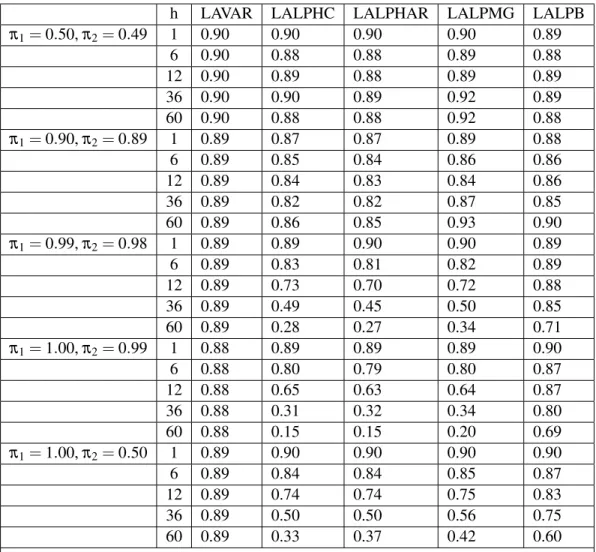
In contrast to Xu (2023) who assumes infinite order DGP, we keep the assumption that the delay order is known to obtain a consistent comparison with other methods. 5) The final method, referred to as LALPB, follows the bootstrap procedure in Montiel Olea and Plagborg-Møller (2021). For the local projection methods, they all lead to undercoverage when at least one of the roots is close to 1 and the horizon is not short, which is consistent with the theoretical and simulation results in Montiel Olea and Plagborg-Møller (2021) and Xu (2023). The results are for the response of the second variable to the reduced first shock.
The results concern the response of the second variable to the first structural shock. The magnitude distortion of the local projection methods is comparable to that for reduced-form impulse responses.
Median length
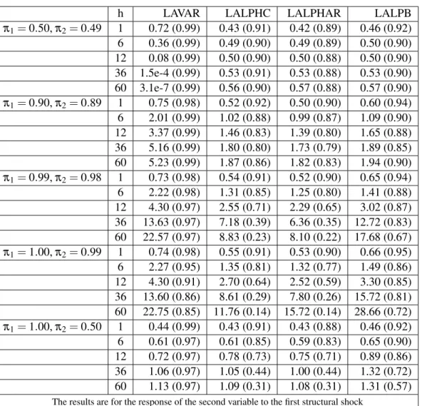
Repeat (3) and (4) until we have enough accepted draws of ΠandΣ. Calculate the upper and lower limits of the structural impulse responses corresponding to these drawings to construct the confidence interval. The results are for the second variable's response to the first structural shock and are reported as "median length (degree of coverage)". First, for a strictly stationary model where π1=0.5 and π2=0.49, the length of our intervals shrinks to 0 as the horizons increase, even though the exact horizon where our method starts has lower length, depends on the persistence of the DGP.
Finally, for our method, as briefly mentioned in the discussion above, the actual coverage rates of the confidence intervals are higher than the nominal rate (and the coverage rates from size studies) for stationary models and slightly lower for very persistent patterns. Finally, when the DGP is very persistent, the magnitude of the impulse responses becomes very sensitive to the model parameters.
Conclusions
For models with roots very close to 1 or exactly 1, the confidence intervals of our method still manage to reach the nominal coverage, except for π1=1 and π2=0.99 at larger horizons, in which case the coverage percentages are still reasonably close to the nominal coverage percentage. rate. Furthermore, when an exact unit root exists, LALPB actually yields larger confidence intervals, with worse coverage rates, compared to our method. The actual confidence set may not be a coherent interval, implying that our confidence intervals may be somewhat conservative.
We find that there is no universally more efficient method, but at very high levels of persistence, our method leads to significantly less coverage distortion than the local projection method, while our confidence intervals have comparable or lower lengths. Furthermore, when the roots are strictly stationary, the confidence intervals from the VAR methods gradually shrink toward length 0 as the horizon increases, while the intervals from the local projection methods do not.
Introduction
For example, in a small-scale structural VAR, a researcher using a short-term recursive identification scheme could perform additional robustness checks by changing the order of the variables. In other words, such an assumption reduces the identification problem of the structural shocks to normalization that does not affect the structural impulse responses to each shock. In terms of independence, structural shocks, by their definition and construction, are intended to be orthogonal and able to span the space of the economy.
In this chapter, we chose to perform the maximum likelihood estimation in Lanne et al. 2017), which assumes a correct specification of the distribution of structural shocks. The first step is to estimate the principal component of the unobserved factors, and the second step, assuming that the distribution of structural shocks is known, performs maximum likelihood estimation (MLE).
Model and identification
Assumptions
This suggests that although their identification scheme is appropriate and standard in the literature, empirical researchers should be cautious about the economic implications and perhaps refer to alternative identification schemes as a robustness check. In principle, non-Gaussian structural errors mean non-Gaussian reduced form errors that can be tested on the data, as for example in Kilian and Demiroglu (2000). In addition to Assumption 2.1, we need assumptions that ensure factor extraction and VAR stationarity.
Factor model) (1) The factors F satisfy E. 2) The factor loadings of the unobserved factors are deterministic and N−1Λ0Λ→ΣΛ, a fixed positive definitive matrix as N→∞. 3) The eigenvalues of the r1×r1matrixΣΛΣF are different. Assumption 2.3. 1) {ft},{εt}and{ut}are three mutually independent groups. In particular, assumption 2.2(1) guarantees that factors are not degenerate and (2) guarantees that all elements of the factors contribute to the variance ofxt, while (3) is a technical assumption to guarantee the uniqueness of the factors. main component procedure.
Identification through non-Gaussianity
Although Gonc¸alves and Perron (2014) provide a weaker set of alternative assumptions, we choose not to adopt them for simplicity. Now the response to the structural shocks is under the alternative set of parameters. The above result shows that the structural impulse response of the observed factor yt, together with the approximate responses of the information variables Xt, is not affected by either the rotation introduced in the first step of the principal component, or the potential permutation and scaling from identification. through non-Gaussianity.
However, we emphasize that this is a statistical identification result rather than an economic result, as the structural shocks do not necessarily have a specific economic meaning. To properly label the structural shocks, as proposed by Lanne et al. 2017), one could inspect the shape and signs of the estimated impulse responses, and refer to a variety of economic theories and intuitions.
Estimation, inference and testing
After obtaining an estimate of the unobserved factors, following Lanne et al. 2017), we consider a maximum likelihood estimation of the VAR model. These assumptions place constraints on the smoothness and tail behavior of the density function, and are similar to assumptions 4 and 5 in Lanne et al. Then the blocks of the Hessian. where it is a special elimination matrix that follows footnote 8 of Lanne et al. 2017), and Krr is the commutation matrix such that Krrvec(A) =vec(A0) for any×rmatrixA.
Forlλ π,t the first term(Ir p+1⊗B∗−1Σ∗−1) does not depend on G, so we consider an element of the second termgt⊗exλ,t(θ∗,ggg†t). The above result, Theorem 2.3, implies that the principal components estimate of the first step does not affect the asymptotic variance of the estimates of the second step.
Simulation
To be more specific, when testing B(1,3) =B(2,3) =0 when there are three factors in total, this should be interpreted as the first two factors not responding simultaneously to the third shock, rather than a shock that does not affect two of the factors. Since we assume that the factor loadings are deterministic, we keep the realization of the factor loadings the same through several Monte Carlo iterations. We focus on the estimation and inference of the structural impulse response of the third factor, i.e.
However, in practice, derivations of impulse responses with respect to parameters, especially shape parameters, can be difficult to evaluate given the choice of distribution. Delta method intervals seem to suffer significantly when T is significantly larger than N, indicating a possible violation of our assumption.

Empirical application
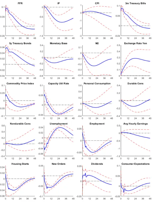
To better compare the results, we use the same data set as in Bernanke et al. Note that this is not a test of the economic identification assumption in Bernanke et al. Alternatively, we derive the factors assuming slow- and fast-moving variables as in Bernanke et al.
To better demonstrate the differences between our results and Figure II in Bernanke et al. 2005), we also plot their point estimates alongside our results in Figure 2.2. Similarly, the effect on the exchange rate also appears to be more persistent compared to Bernanke et al.
Conclusions
Their point estimates are referred to as IRF-BBE, while our point estimates and confidence intervals are referred to as IRF-nonG and CI-nonG. We also provide a comparison of the 90% confidence intervals in Figure 2.3, where their confidence intervals are labeled CI-BBE and our confidence intervals are labeled CI-nonG. The results show that although our test procedure points to problems in the identification strategy of Bernanke et al. 2005), the impulse responses, especially the point estimates, are not significantly different from theirs. However, the lower bounds of the confidence intervals are now negative over all horizons, so there is no longer a price puzzle.
Their two-step estimator produces confidence intervals that are non-negative at least in the very short run, and although their Bayesian estimator does not allow for a price puzzle, the confidence intervals are too wide to be interpreted correctly. We also conduct a simulation study demonstrating the construction of confidence intervals using our proposed estimator, and the results of the study confirm the finite sample validity of our method.
Notations
Changing the international transmission of financial shocks: Evidence from the classical time-varying favar. Journal of Money, Credit and Banking. In Proceedings of the Third Berkeley Symposium on Mathematical Statistics and Probability, Volume 5: Contributions to Econometrics, Industrial Research, and Psychometrics, pages 111–150. On the existence and uniqueness of the real logarithm of a matrix. Proceedings of the American Mathematical Society.
Non-parametric tests for independence: a review and comparative simulation study with an application to malnutrition data in India. Hot money and quantitative easing: the spillover effects of our monetary policy on the Chinese economy.