Essays on the Role of Durables and Financial Frictions in Business Cycles and International Trade
By Dong Cheng
Dissertation
Submitted to the Faculty of the Graduate School of Vanderbilt University
in partial fulfillment of the requirements for the degree of
DOCTOR OF PHILOSOPHY in
Economics August 10, 2018 Nashville, Tennessee
Approved:
Mario J. Crucini, Ph.D.
Gregory W. Huffman, Ph.D.
Atsushi Inoue, Ph.D.
Hyunseung Oh, Ph.D.
David C. Parsley, Ph.D.
To my parents, who supported me all the things great and small.
ACKNOWLEDGMENTS
I would like to extend sincere thanks to the many people, in many places, who generously contributed to the work presented in this dissertation.
Special mention goes to my caring and enthusiastic supervisor, Mario J. Crucini. He provided invaluable encouragement and guidance in my writing of this dissertation. My Ph.D. has been a wonderful experience with his help. I thank Mario wholeheartedly, not just for the tremendous academic guidance, but also for giving me a vast of opportunities. He supported me many times using his research funds, which financed my trips for presenting papers, attending conferences, interacting with great economists, and exploring the other parts of the world. I also learnt so much by working with him on our joint projects. He is always ready to help and keeps optimistic in face of all challenges. His kindness and positive attitude have greatly encouraged me to overcome difficulties that emerged in the process of writing this dissertation.
I am also appreciative to Gregory W. Huffman, Atsushi Inoue, Hyunseung Oh and David C.
Parsley, who served as my dissertation committee members. They provided great comments and feedbacks during my presentations and academic talks between us. I even got very useful advice from then on how to behave well in job market interviews and flyouts.
Profound gratitude goes to Zhongzhong Hu, Joel Rodrigue, Yong Tan and Jian Yu, who are my coauthors in multiple papers. I learnt a lot of innovative ideas, cutting-edge skills, positive attitudes and the spirits of teamwork from them. Special mention goes to Joel Rodrigue, who helped me tremendously by providing comments on my dissertation and exchanging ideas for our joint work.
He showed genuine interests to work with Ph.D. students like me and always encouraged us to explore the frontier.
I would also want to thank many other professors at Renmin University of China and Vanderbilt University for encouraging and supporting me. My M.A. thesis advisor, Yanbin Chen, inspired me to pursue a Ph.D. Tong Li and Mattias Polborn supported me a lot in my searching for jobs.
Federico Gutierrez and Pedro Sant’anna provided great comments during my job practice talk.
Sincere thanks also go to a great number of friends, including Hayri Alper Arslan, Hui (Gracie) Hao and many others, for their help and encouragement. I learnt a lot by interacting with them.
Moreover, gratitude goes to the Walter M. Noel Dissertation Fellowship and a Kirk Dornbush Summer Research Grant for financial assistance.
Finally, but by no means least, massive thanks go to my family, for their almost unbelievable support. Bean and our lovely cat Dill have always been standing with me and giving me enormous support. My mom and dad are the greatest parents for me and give my endless love. They are the most important people in my world and I dedicate this dissertation to them.
TABLE OF CONTENTS
Page
DEDICATION . . . ii
ACKNOWLEDGMENTS . . . iii
LIST OF TABLES . . . viii
LIST OF FIGURES . . . x
INTRODUCTION . . . 1
Chapter 1 Housing Boom and Non-housing Consumption: Evidence from Urban Households in China 4 1.1 Introduction . . . 4
1.2 Background . . . 10
1.2.1 Housing Markets in China . . . 10
1.2.2 Higher-Education Expansion in China . . . 12
1.3 Data and Measurement . . . 14
1.3.1 Urban Household Survey . . . 15
1.3.2 Variable Construction . . . 16
1.3.2.1 Household-level Variables . . . 16
1.3.2.2 County-level Variables . . . 19
1.3.3 Summary Statistics . . . 21
1.3.3.1 Household-level Descriptive Statistics . . . 22
1.3.3.2 County-level Descriptive Statistics . . . 25
1.4 Regression Specification and Identification . . . 26
1.4.1 Baseline Regression Specification . . . 26
1.4.2 Endogeneity of Housing Price Movement . . . 32
1.4.3 Identification with Instrumental Variables . . . 35
1.5 Empirical Results . . . 41
1.5.1 Baseline Estimation Results . . . 42
1.5.2 Heterogeneous Consumption Response . . . 46
1.5.2.1 Homeownership Matters . . . 46
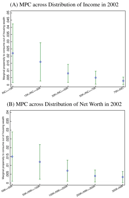
1.5.2.2 Heterogeneity across Income and Wealth Distribution . . . 48
1.5.2.3 The Role of Collateral Constraint . . . 49
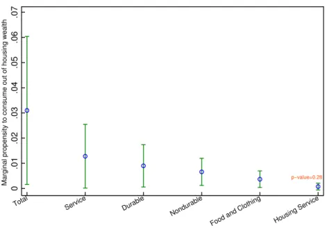
1.5.2.4 Heterogeneity across Categories of Consumption . . . 51
1.6 Robustness Checks . . . 52
1.6.1 Prefecture-level Regressions . . . 52
1.6.2 Error-in-variable Estimation Results . . . 54
1.6.3 Hedonic Housing Price . . . 55
1.6.4 Panel Regression and Habit Formation . . . 56
1.7 Conclusion . . . 58
2 The International Diffusion of the Automobile from 1913 to 1940 . . . 60
2.1 Introduction . . . 60
2.2 Product Diffusion in Historical Data . . . 63
2.3 The Data . . . 64
2.4 The Model . . . 66
2.4.1 Theoretical Diffusion Curve . . . 68
2.4.2 Theoretical Wedge . . . 69
2.5 Estimating Stocks . . . 71
2.6 Reduced Form Quantity Dynamics . . . 74
2.6.1 Diffusion as Measured by the ROW Aggregate . . . 75
2.6.2 Diffusion by Country . . . 75
2.7 Reduced Form Price Dynamics . . . 76
2.8 Results . . . 77
2.8.1 Nation-Specific Theoretical Wedge . . . 78
2.8.2 Wedge Accounting . . . 79
2.8.3 Interwar Commercial Policy . . . 80
2.8.4 Trade Costs . . . 81
2.8.5 Exchange Rate Arrangements . . . 82
2.8.6 Cross-sectional versus Time Series Variation . . . 83
2.8.7 Comparison of Theoretical and Empirical Wedges . . . 83
2.9 Conclusion . . . 85
3 Time-Varying Impacts of Financial Credits on Firm Exports: Evidence from Export Deregulation in China . . . 87
3.1 Introduction . . . 87
3.2 Policy Background and Data Description . . . 91
3.2.1 Policy Background . . . 92
3.2.2 Hypotheses . . . 93
3.2.3 Data Description . . . 95
3.3 Measurement and Empirical Methodology . . . 99
3.3.1 Construction of Key Variables . . . 99
3.3.2 Empirical Methodology . . . 100
3.4 Baseline Results and Robustness Checks . . . 104
3.4.1 Difference-in-Differences Estimates . . . 105
3.4.2 Difference-in-Difference-in-Differences Estimates . . . 108
3.4.3 Utilization of Finance Matters . . . 111
3.4.4 Robustness Checks . . . 113
3.5 Conclusion . . . 116
BIBLIOGRAPHY . . . 118
APPENDICES . . . 130
A.1 Appendices for Chapter 1 . . . 130
A.1.1 Figure Appendix . . . 130
A.1.2 Table Appendix . . . 136
A.2 Appendices for Chapter 2 . . . 152
A.2.1 Figure Appendix . . . 152
A.2.2 Table Appendix . . . 158
A.2.3 Data Appendix . . . 163
A.2.3.1 Trade Data . . . 163
A.2.3.2 Macroeconomic Data . . . 163
A.2.3.3 Census of Manufacturers Data . . . 164
A.2.4 Estimation Appendix . . . 165
A.2.4.1 Trade Costs . . . 165
A.2.5 Historical Appendix . . . 167
A.3 Appendices for Chapter 3 . . . 170
A.3.1 Figure Appendix . . . 170
A.3.2 Table Appendix . . . 172
A.3.3 Data Appendix . . . 191
A.3.3.1 Matching Procedure for Manufacturing and Customs Data . . . 191
LIST OF TABLES
Table Page
A.1 County-level summary statistics for benchmark UHS data . . . 137
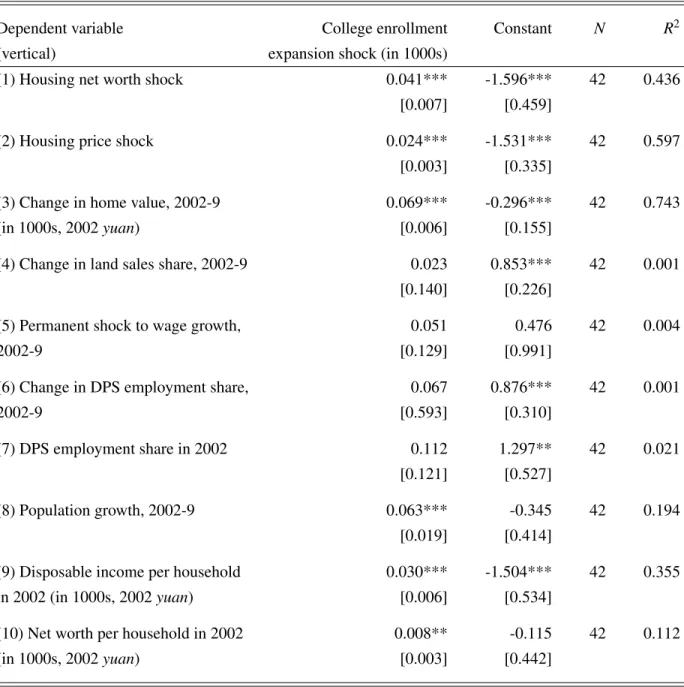
A.2 College enrollment expansion shock as a source of exogenous variation . . . 138
A.3 Household-level log housing price and log consumption . . . 139
A.4 Household-level home value and consumption . . . 140
A.5 County-level housing net worth/housing price shock and consumption growth . . . 141
A.6 County-level average MPC out of housing wealth . . . 142
A.7 County-level log housing price and household-level log consumption for renters . . 143
A.8 Heterogeneous average MPC out of housing wealth across housing leverage ratios 144 A.9 Prefecture-level housing net worth shock and consumption growth . . . 145
A.10 Prefecture-level average marginal propensity to consume out of housing wealth . . 146
A.11 EIV estimation for county-level housing net worth shock and consumption growth 147 A.12 EIV estimation for county-level average MPC out of housing wealth . . . 148
A.13 Prefecture-level elasticity estimation with alternative housing price . . . 149
A.14 County-level elasticity estimation with panel regression . . . 150
A.15 County-level average MPC out of housing wealth with panel regression . . . 151
A.16 Estimated rest-of-the-world diffusion curves with logistic function . . . 158
A.17 Estimated diffusion curves by country with logistic function . . . 158
A.18 Estimated inflection points and long-run adoption levels . . . 159
A.19 Reduced form price dynamics . . . 160
A.20 Ad valorem equivalent tariffs on passenger automobiles . . . 161
A.21 Theoretical and empirical wedges and their components with elasticity = 4 . . . . 162
A.22 Basic statistical summary of the ASIP dataset . . . 172
A.23 Basic statistical summary of the customs dataset . . . 172
A.24 Three types of firms in the matched dataset . . . 173
A.25 DID estimation for export value with internal finance . . . 174
A.26 DID estimation for export value with external finance . . . 175
A.27 DID estimation for TFPR with internal finance . . . 176
A.28 DID estimation for TFPR with external finance . . . 177
A.29 DDD estimation for export value with internal finance . . . 178
A.30 DDD estimation for export value with external finance . . . 179
A.31 DID estimation for efficiency of finance usage . . . 180
A.32 DID estimation for export value with internal finance and alternative fixed effects . 181 A.33 DID estimation for export value with external finance and alternative fixed effects . 182 A.34 DID estimation for TFPR with internal finance and alternative fixed effects . . . . 183
A.35 DID estimation for TFPR with external finance and alternative fixed effects . . . . 184
A.36 DDD estimation for export value with internal finance and alternative fixed effects 185 A.37 DDD estimation for export value with external finance and alternative fixed effects 186 A.38 DID estimation with an alternative IV for switching . . . 187
A.39 DDD Estimation with an alternative IV for switching . . . 188
A.40 DID estimation for export value with finance proxy . . . 189
A.41 DDD estimation for export value with finance proxy . . . 190
LIST OF FIGURES
Figure Page
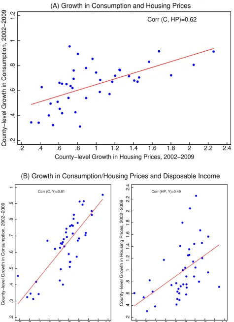
A.1 Correlation patterns: consumption, housing prices, and income . . . 130
A.2 College enrollment and college graduates . . . 131
A.3 Geographic span of benchmark sample from the UHS . . . 132
A.4 Household-level correlation patterns: consumption and housing . . . 133
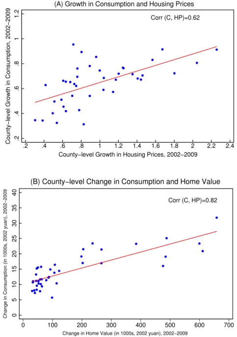
A.5 County-level correlation patterns: consumption and housing . . . 134
A.6 Heterogeneity in MPC: income and wealth distribution . . . 135
A.7 MPC across various categories of consumption . . . 136
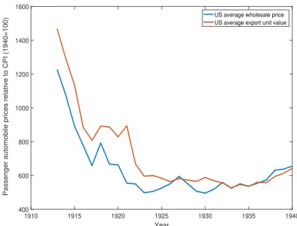
A.8 Domestic prices and export unit values of U.S. passenger automobiles . . . 152
A.9 U.S.and rest-of-the-world passenger automobile registrations per 1,000 persons . . 152
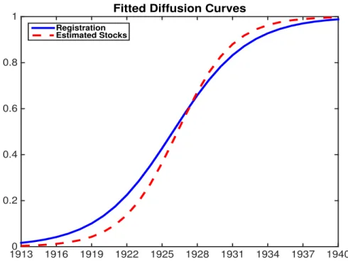
A.10 Simulated diffusion using U.S. export unit values . . . 153
A.11 Theoretical wedges and markup of U.S. EUV over U.S. domestic prices . . . 154
A.12 Automobile stock estimates and their components . . . 155
A.13 Philippine Islands automobile stock estimates . . . 156
A.14 Estimated diffusion using CHAT registration measure and stock-flow estimate . . . 156
A.15 Distribution of EUV deflated by the U.S. CPI . . . 157
A.16 Cross-country distribution of theoretical and empirical wedges . . . 157
A.17 Share of PDEs and average productivity of new switchers . . . 170
A.18 Four measures of firms’ efficiency in utilizing finance . . . 171
INTRODUCTION
Financial frictions are important features of the economy and yet their role in shaping business cycle dynamics and the pattern of international trade is incompletely understood. The role of finan- cial friction is even more crucial when durables are explicitly built into the macroeconomic models because they are big-ticket items. Durables also amplify business cycles through the stock-flow relation because a given percentage change in the desired stock requires a much larger percent- age change in the flow. In the globalized world, trade flows, especially durables, are substantially more volatile than domestic economic aggregates like GDP. Therefore, investigating the role of durables and financial frictions in closed and open economy settings is very important for under- standing economic fluctuations and trade dynamics. Using rich microeconomic and historical data, this dissertation proposes new empirical and theoretical approaches to quantify the importance of durables and financial frictions in three different settings. The first chapter explores the response of non-shelter consumption to shocks from the housing sector, where homes are durable goods that have the unique feature that they also serve a collateral for loans. We develop a novel instrumental variable for local housing price movements to achieve identification. We pay close attention to the role of collateral constraints and show that their presence increases the consumption response. In the second chapter, we investigate the diffusion of a durable good, the automobile, from the United States to the rest of world through international trade. We collect archival data to document the diffusion pattern, and then rely on international price frictions, including markups, tariffs, trade costs, and the Penn effect, to explain the much lower adoption rates of automobiles abroad, com- pared to the U.S. The third chapter examines the heterogeneous and time-varying effects of finance on firms’ exporting performance. We apply panel-data DID and DDD methods to comprehensive microeconomic data from China’s manufacturing sector. We show that both internal and external finance have positive impacts on the intensive margin of firms’ exports when firms switch from in- direct to direct exporting, and even larger positive impacts when the switch occurs in the post-WTO accession period during which government restrictions on direct exporting was removed.
Chapter 1 studies the response of non-housing consumption to housing price movements in urban China, which has been enjoying a real estate boom ever since 2003. Using Urban House- hold Survey data over the period 2002-2009, we estimate an elasticity of consumption with respect to housing price of 0.06 to 0.07 for homeowners. Moreover, we find that the average marginal propensity to consume out of housing wealth is 0.025 to 0.03. The estimates are economically significant because they imply that the increase in consumption induced by housing apprecia- tion during 2002-2009 amounts to 14%-17% of current consumption in 2009 for a representative homeowner. We employ a novel instrumental variable associated with China’s higher-education expansion between 1998 and 2005 to ensure that these estimates are causal effects. As for renters, we show that their consumption response to housing shocks is insignificant. We further reveal that the marginal propensity to consume is larger for homeowners residing in poorer and more collat- eral constrained cities. Greater durability or a higher income elasticity of a consumption category amplifies homeowners’ consumption response to housing shocks.
The first half of the twentieth century provides an unparalleled opportunity to explore the im- pact of technological innovation in the worldwide diffusion of a new and highly traded good, automobile, because the United States was dominant in both production and trade of passenger automobiles. In Chapter 2, we scrape historical data on quantity and value of passenger vehicles exported from the United States to approximately 80 destinations, annually from 1913 to 1940. We model the rise of the automobile from global obscurity to a fixed point which depends on per capita national wealth, and with the transition path depending on the evolution of the relative price of the automobile and its pass-through to destination markets. We then conduct wedge accounting for international price frictions, including markups, tariffs, trade costs, and the Penn effect, to explain the gaps of adoption levels between the U.S. and other countries.
Chapter 3 investigates the heterogeneous and time-varying effects of financial credits on firm level export performance. China’s WTO accession leads to trade deregulation, which allows do- mestic private firms with low registered capital to switch their export mode from indirect (through intermediaries) to direct exporting. Using a comprehensive data set of Chinese manufacturing firms
and employing a difference-in-differences approach (DID), we find that financial credits improve firm-level exports and productivity more for firms that switch from indirect to direct exporting than continuous indirect exporting firms. Further, we employ a difference-in-difference-in-differences (DDD) approach and find that improvements in firm-level internal and external finance have larger positive impacts on firm export values in the post-WTO accession period, conditioning on the firm switching from indirect to direct exporting. The time-varying impact may suggest an export distortion in China before its WTO accession, which prevents more productive but financially con- strained private domestic firms from direct exporting.
CHAPTER 1
Housing Boom and Non-housing Consumption: Evidence from Urban Households in China
1.1 Introduction
When homeowners experience an increase in the market value of their homes due to macroe- conomic or local sources of variation, how does their non-housing consumption respond? This question is important for understanding how wealth shocks translate into business cycle fluctua- tions, and has strong policy implications with regard to large swings in asset prices. Existing studies (e.g. Mian et al., 2013; Kaplan et al., 2016) show that there is a large consumption response to housing price movements in developed economies, especially during economic crises.1 However, less is known about the consumption response in a developing economy like China that has been enjoying a decade-long boom in housing markets.2
In this paper, we estimate the causal impact of housing shocks on consumption in China. Two features make China a quite different setting from developed economies for evaluating the con- sumption response. First, less developed financial markets force households to save a large share of current income against future uncertainties, hence limiting the extent of consumption response to perceived appreciation in home values. Second, following a decade of consistent price appreci- ation in housing markets, households may expect a continuation and this amplifies consumption response to the current price rise. These competing forces (among others) may lead to either a larger or smaller consumption response than those found in developed economies. Hence, our work avoids the extrapolation of existing estimates to economic environments where they may be inappropriate while providing additional lessons on the general boom-bust cycle of housing.
1Mian et al. (2013) refer to housing price movements as housing shocks to reflect the fact that they explore how exogenous variation in housing price movements affects household consumption using the instrumental variable method. We follow their terminology in this study because we also construct an exogenous source of variation in housing price movements.
2Since 2003, Chinese housing markets have been growing rapidly and steadily. Glaeser et al. (2017) document that, during 2003-2014, real housing prices in China rose by over 10% per year, and Chinese real estate developers added around 100 billion square feet of residential space. Even the U.S. housing boom between 1996 and 2006 pales in comparison to the great Chinese housing boom, with real housing prices growing by 5% per year.
Exploring the casual effect of housing shocks on consumption faces the challenge of isolating multiple channels that could explain any observed relationship between the two variables. One branch of papers have employed a calibrated model of consumption and housing to evaluate the consumption response, and find that the elasticity of consumption with respect to housing price is positive and significant. Early studies like Campbell and Cocco (2007) and Attanasio et al. (2011) employed variants of the partial equilibrium life cycle model to explore consumption responses, while recent papers (e.g. Berger et al., 2017; Kaplan et al., 2017) have switched to introducing housing into (general equilibrium) incomplete market models with heterogeneous agents. Another branch of papers are more reduced-form, and while differences in estimation strategies and data leads to a broad range of estimates for the consumption response, the median response across these studies is large, positive, and statistically significant. Early reduced-form studies using aggregate data (e.g. Carroll et al., 2011) found it hard to construct a reliable source of exogenous variation in housing price movements to isolate the impact of housing shocks on consumption. Recently, relying on the housing supply elasticity constructed in Saiz (2010) as an instrumental variable for local housing price movements, Mian et al. (2013) improved the situation when exploiting the consumption response with data at county and zip-code levels.3
The challenge of identification also plagues our empirical work when we extend the studies on consumption effects of housing shocks to a developing economy like China that has been en- joying a decade-long housing boom. In Figure A.1, we plot correlation patterns between real growth in county-level consumption, housing prices, and disposable income during 2002-2009.
Panel (A) clearly displays that real consumption and real housing prices rose dramatically in urban China between 2002 and 2009. The two growth rates also show strong positive correlation across locations, suggesting a positive effect of housing appreciation on consumption. However, the ob-
3Though recent reduced-form studies explore the consumption response to both housing price and home value (housing wealth) movements, they focus on changes in home value driven by housing price movements (e.g. Mian et al., 2013; Kaplan et al., 2016). Hence, the changes in quantity of housing are not considered. It makes sense to isolate changes in home value driven by housing price movements because housing prices tend to be more exogenous than housing quantity for households once they buy homes. This treatment also implies that it is appropriate to instrument home value changes with the instrumental variable for housing price movements, as Mian et al. (2013) have done in their study.
served correlation may be ascribed to a common outside factor that moves both the growth rates of consumption and housing prices in the same direction. For instance, Panel (B) indicates that the spectacular income growth could boost consumption and housing price simultaneously through increased demand for non-housing consumption and housing services. As a consequence, any un- observed permanent income shock might lead to the positive correlation between consumption and housing price growth. To avoid misattribution like this, we need to find an exogenous source of variation in housing price movements to clearly identify the causal effect of housing shocks on consumption. It is beyond the scope of this paper to construct geography-based long-run housing supply elasticities as Saiz (2010) using geographic information system (GIS) techniques. Instead, we develop an alternative source of exogenous variation in housing price changes that takes advan- tage of an arguably natural experiment in China and originates from the demand side of housing markets.
We exploit China’s higher-education expansion between 1998 and 2005 to construct an instru- mental variable for housing price movements during 2002-2009.4 The higher-education expan- sion is conceivably a natural experiment and exogenous to concurrent economic growth trend in China (Che and Zhang, 2017). We construct college enrollment expansion shock as an instrumen- tal variable for city-level housing price movements between 2002 and 2009 through the multipli- cation of initial number of city-level higher-education institutions in 1998 (prior to 1999 when higher-education expansion was introduced) and province-level college enrollment expansion dur- ing 1998-2005.5 The choice of initial number of higher-education institutions prior to college enrollment expansion mitigates the endogeneity concern that more colleges are built for expansion in areas that are expected to grow faster, while the province-level college enrollment expansion further helps us to avoid endogenous expansions at the city level.
Our instrumental variable is predictive of local (city-level) housing price increases over the
4Our approach to constructing an instrumental variable for housing price movements is inspired by the recent work of Chen and Zhang (2016) who utilize the same higher-education expansion to explain housing price increases in China. They find that the college enrollment expansion leads to an increase in local demand for housing that can account for around 12%-20% of housing price changes in China during 2002-2009.
5The timeline of events is plotted in Section F of this paper’sOnline Appendix. It clearly defines our sample period, the period of higher-education expansion, and the period we employ to construct our instrumental variable.
period 2002-2009 mainly through local accumulation of college graduates who enjoyed substan- tially high wage premiums as skilled workers. When a city experiences a larger college enrollment expansion shock, it accumulates more local human capital in the form of skilled workers once a larger number of college students graduate and stay locally to work after four years of college study.6 This further translates into higher demand for local housing and hence (ceteris paribus) strongly appreciates local housing prices because Chinese college graduates enjoy high wage pre- mium and have strong demand for housing.7 By checking correlation patterns, we show that the college enrollment expansion shock is significantly positively correlated with housing shocks, and orthogonal to major endogeneity concerns on housing price movements that we could expect in the context of China, like permanent income shocks and trade liberalization shocks to the domestic private sector.8
We employ microeconomic data from Urban Household Survey (UHS) to estimate the causal response of household consumption to housing price movements in China. The UHS is a nation- wide survey conducted by China’s National Bureau of Statistics (NBS) on an annual basis, and we have access to a subset of data covering 6 provinces over the period 2002-2009. We construct consumption (excluding consumption of housing services), housing, and other socioeconomic vari- ables at both household and city (county/prefecture) levels. The comparison of summary statistics at the household level with existing studies cross validates the representativeness of our sample.
Rich cross-sectional variation across households is further used to show the strong positive corre- lation between consumption and housing price or housing wealth. In contrast, we rely on city-level
6According to data from the National Bureau of Statistics, the annual four-year college graduation rate during 2002-2009 was between 95% and 97% in China. This is much higher than the case in the United States. Aggregate data from the National Center for Education Statistics (NCES) show that U.S. annual four-year college graduation rate was 35%-40% during 2004-2014.
7For instance, Han et al. (2012) document that wage premium for college graduates (in comparison to high school dropouts) increased from 60% to 80% in urban China during 2002-2008. Though there exists a concern that a sharp expansion in college enrollment (through the lowering of admission scores) could lead to a remarkable drop in the quality of college graduates and hence a decline in wage premium for skilled workers (mainly college graduates), evidence from Han et al. (2012) strongly falsifies this narrative. As Han et al. (2012) suggest, this puzzle can be reconciled by the fact that China’s accession to the World Trade Organization (WTO) created massive demand for skilled workers. Consequently, the increased demand overcome the decline in quality and resulted in a rise in wage premium for college graduates.
8More intuitively, for the relevance of our instrumental variable, we find a simple elasticity showing that local housing prices on average go up by 1.4% when local college enrollment expands by 10%.
regressions to estimate the causal effect because the instrumental variable is available only at the city level.
With the help of the novel instrumental variable (college enrollment expansion shock), we es- timate an elasticity of consumption with respect to housing price of 0.06-0.07 for homeowners, or equivalently an elasticity of 0.12-0.13 with respect to housing wealth.9 We also find that the average marginal propensity to consume (MPC) out of housing wealth is 0.025 to 0.03. The MPC estimate is quantitatively consistent with the elasticity estimate, given that the average ratio be- tween housing wealth and consumption was 6.8 for homeowners during our sample period.10 The estimated consumption response is economically significant. Specifically, the MPC estimate indi- cates that the increase in consumption induced by housing appreciation during 2002-2009 equates to 14%-17% of current consumption in 2009 for a representative urban homeowner. In addition, we show that our baseline results are robust to error in variables that emerges when we proxy pop- ulation means with sample averages to implement city-level analysis. They also survive robustness checks on hedonic housing prices and habit formation in consumption.
In addition to the economically significant average consumption response to housing shocks, we reveal that there exists considerable heterogeneity in consumption response along several di- mensions, including homeownership, income/wealth status, degree of collateral constraint, and durability or income elasticity of consumption goods. As for renters, the estimation results suggest that their consumption response to housing shocks is insignificant. Furthermore, we find that the MPC out of housing wealth is higher for households residing in poorer and more collateral con- strained cities. Greater durability or a higher income elasticity of consumption goods also amplifies the consumption response.
Our paper mainly contributes to the empirical studies on household consumption response to
9The equivalence is implied by the fact that the average share of housing wealth in total net worth was around 56%
in 2002 for homeowners (multiplying 0.12-0.13 by 0.56 produces 0.06-0.07).
10Note that the elasticity with respect to housing wealth equals to the product of the estimated MPC out of housing wealth and the ratio of housing wealth to consumption. Therefore, the MPC estimate implies an elasticity with respect to housing wealth of 0.17-0.21 (multiplying 0.025-0.03 by 6.8). The magnitude difference between 0.17-0.21 and 0.12-0.13 is mainly ascribed to the fact that we add quite different controls when estimating elasticity and MPC.
housing price changes.11 It is most closely related to the recent papers by Mian et al. (2013) and Kaplan et al. (2016) that empirically investigate the causal impact of housing price bust on consumption collapse during the 2006-2009 financial crisis. Employing U.S. data at the county or Core-Based Statistical Area (CBSA) level, they find that the elasticity of consumption with respect to housing price is around 0.2. Compared with their estimates, we discover an elasticity of 0.06 to 0.07 for homeowners in a large developing economy that has been experiencing a decade- long housing boom. Besides the asymmetry induced by the concavity of consumption function in boom and bust of asset prices, we conjecture that the smaller consumption response of Chinese urban households might also be ascribed to several macroeconomic features unique to China.12 It includes but is not necessarily limited to the underdevelopment of financial markets and strong precautionary saving motives due to uncertainties stemming from China’s transition to a market economy. Moreover, unlike Mian et al. (2013) and Kaplan et al. (2016), we separate homeowners from renters by taking advantage of microeconomic data. This enables us to straightforwardly assess the role of homeownership, which implicitly reflects the importance of wealth effect and collateral constraint channel.
The rest of the paper is structured as follows. We start with the introduction of background information on Chinese housing markets and higher-education expansion in Section 2. We then present data, variable construction, and summary statistics in Section 3. Section 4 describes base- line regression specifications and deals with endogeneity in housing price movements. Main em-
11Our work is also related to a large literature that employ more structural techniques to study the response of consumption to housing price movements. Good examples include Carroll and Dunn (1998), Campbell and Cocco (2007), Attanasio et al. (2011), Berger et al. (2017), and Gorea and Midrigan (2017). In a broader sense, this paper echoes the empirical studies that investigate the macroeconomic implications of housing wealth from the firm side as well. See, among many others, Chaney et al. (2012), Bahaj et al. (2016), and Catherine et al. (2017).
12Unlike existing studies that attempt to understand the sharp decrease in household consumption following a finan- cial crisis (Jensen and Johannesen, 2016) or a bust in asset prices (Mian et al., 2013; Kaplan et al., 2016), our study explores the contribution of a asset market boom to consumption growth. As suggested by the work of Carroll and Kimball (1996), households with precautionary saving motives have an optimal consumption function that is concave in wealth, when there is uncertainty in labor productivity and asset prices. Hence, we expect an asymmetry in con- sumption response to positive and negative housing wealth shocks. Starting with the same initial housing wealth, an increase in housing wealth will have a smaller impact on consumption than a decline in housing wealth of the same magnitude. The expected less responsive consumption in the boom case also helps us to explain the finding that our elasticity of consumption with respect to housing price is smaller than the elasticity Mian et al. (2013) obtain using U.S. data during the crash period of 2006-2009.
pirical results of this study are reported in Section 5. Robustness checks for the baseline regression results are presented in Section 6. Section 7 concludes.
1.2 Background
We present in this section the background information on the urban housing market and higher- education expansion in China. We first show how institutional changes contributed to the emer- gence of a decade-long housing boom in the early 2000s. Then we introduce the higher-education expansion that started from 1999, against the backdrop of several adverse economic conditions.
The higher-education expansion generated a college enrollment boom, which is employed by this study as a novel instrumental variable for housing price movements.
1.2.1 Housing Markets in China
A great housing boom has been built up ever since China abolished the welfare-oriented public housing allocation system and established formal housing markets. The decade-long housing boom then provides us a unique setting to explore how consumption responds to substantially positive housing shocks.
Housing markets in China are nascent, not formally established until the late 1990s. Before 1978, housing was exclusively provided by the public sector and distributed to households via the working unit-employee linkage. Any institution or organization where people work could be counted as a working unit, including but not limited to enterprises, educational establishments, and government agencies. The working units provided free housing (which was allocated by the public sector) to reward their employees as a form of in-kind compensation. Owing to insufficient funds, an expanding population, and an inefficient allocation system, per capita residential space was very low for Chinese urban households during 1949-1978. In 1978, it was only 3.6 square meters, even lower than that in 1950 (4.5 square meters) when the People’s Republic of China was newly founded.
Starting from 1978, the reform and opening-up policy triggered a series of institutional changes
in the provision of housing. In September 1978, Deng Xiaoping (the paramount leader of China between 1978 and 1989) first proposed that the central government should incentivize private sec- tor to provide housing. His guidance facilitated the State Council to formulate a commercialization policy of housing in June 1980, which granted individuals the rights to purchase homes. In 1982, the central government started a pilot program in four cities to subsidize the purchase of housing from the public sector by households. It primarily aimed to delink housing provision from employ- ment (working units). A milestone was reached in 1988 when Chinese constitution was amended to allow for trading use rights of land, which also laid legal foundations for the marketization of hous- ing in China.13. Broader and more profound housing reform was proposed in July 1994, including subsidizing private purchase of housing, establishing the commercialization and marketization of housing provision, and fostering housing credit markets.
In July 1998, the central government abolished the public housing allocation system and guided individuals to acquire housing, “commodity houses”, from housing markets. This marked the es- tablishment of housing markets in China. Hence, Chinese housing markets are very nascent when compared with mature markets in most developed economies.14Also in 1998, to mitigate negative economic shocks from the 1997 Asian Financial Crisis, the central government established housing
13The situation continues to this day. Only the use rights of land is allowed for transactions in China. The land, by the Chinese constitution, is state owned. Local governments sell leases of land for residential use to real estate developers with a maximum length of 70 years. The leases of land use rights can be traded freely, as long as they do not expire. As pointed out by Glaeser et al. (2017), it is still unclear what the government will do when those use rights expire. Even though there is massive uncertainty in the protection of private property rights pertaining to housing which is built on land that is state owned and has an expiration date for use rights, the central government is taking measures to reduce this risk. Li Keqiang, China’s current premier minister, responded to a reporter question in a recent congress news conference in March 2017 that the State Council is formulating a new policy that allows households to renew leases.
14Though housing prices are market equilibrium prices after the establishment of housing markets, Chinese local governments play an important role in determining housing prices. Since houses and land are closely related, the institutional background on land also affects housing prices. In urban China, land are publicly owned by governments, only use rights of land is allowed for transactions. The typical procedure of land use rights trading goes like this: a local government prepares a piece of land that is leased for residential use with a maximum length of 70 years; next the local government sells the lease to real estate developers mainly through auctions; then developers build houses on the leased land and transfer the lease to households when selling houses to them, notice that land costs prepaid by developers have been factored into selling prices of houses; then households transfer the lease to other households if they decide to sell their houses, note that the depreciated value of lease has been factored into selling prices of houses by households. Considering that land prices accounted for over 40% of housing prices during 1998-2015, it is thus natural for us to expect that local governments can substantially affect equilibrium housing prices in housing markets, simply by controlling the supply of land and thus land prices. Section A of this paper’sOnline Appendixprovides more detailed discussion on housing markets and land supply in urban China.
sector as a new engine of economic growth and a pillar industry for the economy, which substan- tively raised economic status of housing sector. Supporting measures, including subsidizing resi- dential mortgages and broadening construction loans by real estate developers, were implemented to fuel the growth of housing markets. These measures, combined with other institutional changes, were quite effective and contributed to the formation of a housing boom in the early 2000s.15 Dur- ing 2002-2013, home sales have maintained an annual growth of 15%, and the construction of residential housing has grown by 18% annually. Another indicator confirms the housing boom in China during this period, real housing price has risen by over 10 percent between 2003 and 2014.
1.2.2 Higher-Education Expansion in China
To overcome a series of adverse conditions like economic downturns and soaring unemploy- ment, the Chinese central government massively expanded college enrollment during 1999-2005.
The sharp expansion then translated into strong demand for local housing, and hence serving as an effective instrumental variable for local housing price movements.
Like housing, higher education was exclusively provided by the public sector before the eco- nomic reform and market opening-up. The central government adopted the Soviet model to nation- alize higher-education institutions in the early 1950s, and made admission plans for universities or colleges based on the needs of economic development. Since 1952 (even to this day), almost all college students in China have been admitted through a unified national college entrance exam (CEE). The higher-education sector experienced steady growth in the 1950s, yet disrupted and im- peded in the 1960s by the “Great Leap Forward” and in the 1970s by the Cultural Revolution.16
15Many factors have been contributing to the decade-long (from 2003 until now) housing boom in China. To name a few, the strong incentive of local governments to acquire fiscal revenues through the selling of land use rights, the excessive injection of money into housing markets to maintain stably high economic growth, the limited investment vehicles for households due to underdeveloped stock and bond markets, the massively rigid demand for housing by young adults with funding support from parents and extended relatives, and the cultural tradition to own rather than rent homes intensified by the competition among males in the marriage market. Examining relative contributions of those factors requires more rigorous work, which is beyond the scope of this paper.
16Essentially, these two nationwide campaigns severely curtailed the admission of college students and disturbed the normal educational activities in comprehensive universities and specialized colleges. A landmark event was the suspension of college entrance exam in 1966.
It returned to the normal historical track in December 1977 when the college entrance exam was resumed. Between 1978 and 1998, the number of colleges increased from around 600 to more than 1,000, and the college enrollment increased from 0.4 million to 1.08 million (see Li et al., 2014, for more facts).
Although higher education in China experienced steady growth starting from 1978, an unex- pected takeoff occurred in 1999. The sharp expansion was triggered by several unfavorable factors.
First, the 1997 Asian Financial Crisis led to an economic downturn and increase in unemploy- ment. Second, the South Tour Speeches by Deng Xiaoping catalyzed the reform of state-owned enterprises (SOE) into modern corporate entities, which laid off a large number of workers who were inefficient and redundant (Berkowitz et al., 2016). Third, the former prime minister of China, Zhu Rongji, took stringent monetary and fiscal polices in the early 1990s to guide the overheated Chinese economy to a soft landing, which resulted in weak internal demand. To overcome these adverse conditions, the central government adopted the proposal of an economist in Asian Develop- ment Bank (see Che and Zhang, 2017, for more archival details about this proposal) and formulated a higher-education expansion plan that aimed to pull up internal demand, stimulate consumption, promote economic growth, and alleviate employment pressure. The sudden expansion was mainly achieved by lowering CEE admission scores.
The higher-education expansion was conceivably a natural experiment. We plot levels and growth rates of college enrollment and the four-year lead college graduates inFigure A.2to show the unexpected expansion. Note, in particular, the sharp increase in college enrollment of 0.51 million in 1999. The total number of newly enrolled college students reached around 1.6 million, which was a 47.3% rise when compared to that in 1998. The massive expansion continued into the early 2000s, with college enrollment increasing by 38.1% in 2000, 21.6% in 2001, and 19.5% in 2002. On average, the growth rate of college enrollment was as high as 25.1% between 1999 and 2005. It is an extraordinary expansion when we compare it with the average enrollment growth during 1996-1998, that is, 25.1% versus 5.4%. The expansion substantially slowed down starting from 2006, with the annual growth rate dropping from 12.8% to 8.2%. The boom in college enroll-
ment since 1999 translated into a boom in college graduates since 2003, where the four-year gap reflects the typical length of college study in China. College graduates rose by 40.4% in 2003 and kept a growth rate of more than 20% for four years during 2003-2006. Average growth in college graduates between 2003 and 2009 was as high as 22.3%. In this study, we employ the arguably exogenous college enrollment expansion (see Che and Zhang, 2017, and Knight et al., 2017, for more arguments on exogeneity of the higher-education expansion) between 1998 and 2005 to char- acterize increased local demand for housing over the period 2002-2009, and hence utilize it as an instrument for local housing price movements between 2002 and 2009.
There are two channels through which the central government managed to deal with such a massive expansion in college enrollment. At the intensive margin, the existing higher-education institutions were quite spacious to accommodate an abrupt rise in enrollment. Aggregate data show that the average student-faculty ratio was around 7 to 1 in 1998. At the extensive margin, many more higher-education institutions were established. Between 1998 and 2005, the number of higher-education institutions increased from 1,022 to 1,792. An explosive increase occurred in 2001 when around 200 universities and colleges were built in that single year. Meanwhile, more faculty members were recruited. The number of faculty was more than doubled during 1998-2005, from 407,000 to 966,000. Expansion in higher-education institutions and faculty members further increased the demand for local housing, hence fueling the growth of local housing prices. Con- struction of new institutions generated fierce competition for land against residential developers, and the newly recruited faculty members had strong purchasing power for housing with their rela- tively high income. More higher-education institutions within a city also attracted more in-migrants via the externality of local human capital accumulation, which then created additional demand for local housing.
1.3 Data and Measurement
We employ Chinese microeconomic data from the Urban Household Survey to explore con- sumption response to housing price/home value movements. Non-housing consumption, housing,
and other socioeconomic variables are constructed at both household and county levels. We then present summary statistics of primary variables. The comparison of summary statistics with exist- ing studies helps to cross validate the representativeness of our sample.
1.3.1 Urban Household Survey
The dataset we use is from the Urban Household Survey, which is conducted annually by China’s National Bureau of Statistics. The UHS contains extensive information on urban house- holds, such as household size, employment status, detailed income and expenditure, and housing wealth. All surveys are uniformly designed and conducted, and of high quality that is guaranteed by province-level scrutiny and timely reporting starting from base-level survey units. The UHS employs a stratified sampling, which is advantageous to sample each stratum independently. It puts massive emphasis on representativeness of the survey at all stratums, including community, county, prefecture, and province. Besides these features embedded in survey design to seek for randomization and representativeness, the NBS also devises cross-validation procedures at the ag- gregate level to further insure the quality of UHS data. It routinely checks the sample variances of disposable income, total consumption expenditure, and household size to track the change in sampling errors. We put more details on the design and implementation of UHS in Section B of this paper’sOnline Appendix.
The UHS data are proprietary and hard to acquire. We have access to a subset that covers six provinces over the period 2002-2009. The six provinces are: Beijing, Liaoning, Zhejiang, Sichuan, Guangdong, and Shaanxi.Figure A.3 presents the geographic span of our sample. It reveals that these six provinces are well divided and geographically dispersed.Figure A.3 also displays that the counties surveyed within each province are also geographically dispersed. The sample size tends to increase with population and, as such, the number of microeconomic observations at the county level tends to be representative of that county’s aggregate size in population and output.
However, it needs to point out that the UHS samples a disproportionately larger share of population for counties with less population and economic importance to guarantee representativeness. The
representativeness of our dataset is also ensured by the fact that the six provinces in our sample took up a reasonable share of national population (25%), consumption (32%), gross domestic product (33%), and completed residential investment (25%) during the sample period. Our data also has a representative number of cities from all tiers of cities which are categorized according to their importance in population and economic volume, hence generating substantial cross-sectional variation in local housing markets. We cross validate several variables in our sample with the aggregated national counterparts published by the NBS to further test the representativeness of our data. For instance, average household per capita residential space grew from 25.4 square meters to 32.5 square meters during our sample period, while the national average increased from 22.8 square meters to around 30 square meters. More discussion on data availability and representativeness can be found in Section B of this paper’sOnline Appendix.
1.3.2 Variable Construction
Variables on consumption, housing, and other socioeconomic variables like employment, in- come, and wealth are constructed at both household and city levels. In the baseline results, county- level cities which match the boundaries of counties are considered. We employ prefecture-level cities which likewise match the boundaries of prefectures in robustness checks.17 Since the con- struction of variables is similar for the two layers of cities, we only introduce county-level variables in this subsection.
1.3.2.1 Household-level Variables
At the household level, consumption variables can be obtained directly from the UHS data.
Consumption expenditures for over 180 items are recorded. We sum up items to define total con- sumption (Cth), nondurable consumption (Ct,ndh ), durable consumption (Ct,dh ), and service consump- tion (Ct,sh ) using the methodology proposed by the Bureau of Economics Analysis (2015), U.S.
17In China, communities constitute counties, counties constitute prefectures, prefectures constitute provinces, and provinces constitute the nation. Both counties and prefectures can be treated as cities. Therefore, we name counties and prefectures as county-level and prefecture-level cities, respectively.
Department of Commerce. Note t denotes a year, h denotes a household, {nd,d,s}denote non- durables, durables, and services, respectively. Housing consumption is carefully taken care of in this study. We include housing consumption in household-level summary statistics to make sure that our results are comparable to existing studies that employ other sources of microeconomic data. However, to avoid the endogeneity involved in housing consumption, we exclude it from consumption in all household-level regressions.18 We exclude housing consumption when con- structing city-level consumption variables, thus city-level regressions are automatically free of any direct endogeneity caused by the inclusion of housing consumption. More detailed information on the construction of consumption variables can be found in Section C of this paper’s Online Appendix.
Most of the housing variables need to be calculated using recorded variables. In line with Mian et al. (2013) and Kaplan et al. (2016), we are particularly interested in two housing variables: home value and housing price. Home value is needed for us to assess MPC out of housing wealth, while housing price is the main driving force of variation in home value and indispensable for us to assess elasticity of consumption with respect to housing price. Home value (HVht) is well recorded in the data. Housing price (HPth) can be recovered using home value and construction area (in square meters) of the house (CAth), i.e. HPht = HVht
CAht . Unlike Mian et al. (2013) and Kaplan et al. (2016) who focus on county or zip-code level analysis using U.S. data, we cannot construct housing net worth shock or housing price shock as they do at the household level, for the reason that our UHS data do not provide an identifier to track the same households over time. It means that our data are pooled cross-sections, rather than a panel. Nevertheless, we construct housing net worth shock and housing price shock as they do for county- or prefecture-level cities when we aggregate households into geographic cohorts (county/prefecture) to conduct pseudo panel analysis.
Besides home value and housing price serving as primary explanatory variables in regressions, we also construct other housing variables that are indicative of the development of housing markets.
18When housing consumption is included in consumption, an endogeneity problem easily arises in the regression of consumption on housing shocks. There exist lots of unobserved factors that could affect both consumption of housing and housing prices. For instance, a negative permanent income shock tends to depress both consumption of housing and housing prices within a location.
Specifically, we calculate per capita residential space in square meters as the ratio of construction area and household size to show the change in housing conditions for Chinese urban households.
We define monthly housing rent rate in yuanper square meter as the ratio of total monthly rent to the area of the owned house, where total monthly rent is the self-estimated amount that should be paid for the housing service delivered by owned homes. We check the validity of the housing rent rate using the rent rate paid by renters for rental houses. It produces quite similar summary statistics in each year of our sample. We prefer the housing rent rate constructed using owned homes because we can further utilize it to define price-to-rent ratio (i.e. the ratio of housing price to annual rent) at the household level, which may be informative of the likelihood of a housing bubble.
The other household variables we construct mainly serve as controls in our empirical analy- sis, including household characteristics on employment, income, and wealth. Household size is the number of people in the household, recorded in the original data, among which the number of wage earners is the sum of all wage earners in different sectors. The fraction of workers in state-owned enterprises (SOE) measures the share of labor in the public sector. Household income characteris- tics contain total income, disposable income, and the fraction of income from working. Disposable income is the total income net of operation outlays (mostly related to home-owned small business), individual income tax, and social security fees. With annual income information, we can construct a proxy variable for the affordability of homes, the price-to-income ratio, which is defined as the ratio of home value to annual household disposable income.
Measuring household wealth characteristics poses greater challenges because the UHS pro- vides a very limited record of specific household asset information other than home values. We employ detailed information on asset income to recover net worth (NWht). Net worth is defined conventionally asNWht =Fth+HVth−Dth, whereFth are financial assets including cash holdings and bank deposits,Dht is the outstanding debt. Cash holdings are well recorded, and bank deposits can be estimated using the formula Total Banking Interest Income
Weighted Bank Deposit Interest Rate, where the weighted deposit in- terest rate is published by the NBS. Similarly, debt can be estimated using annual interest payments
on outstanding debt and weighted bank loan interest rate from the NBS. Bonds and stocks cannot be recovered because the UHS has no income information for them. As a consequence, we ignore them in this study. We argue in Section C of this paper’sOnline Appendixthat dealing with bonds and stocks in alternative ways does not alter our main results.
1.3.2.2 County-level Variables
County-level variables are constructed by aggregating corresponding variables at the household level. We employ sample averages within each county for aggregation, hence abstracting from local demographic transitions and focus on economics behaviors. We keep counties or prefectures that have observations in both 2002 and 2009, for the reason that we need to construct changes and growth rates of variables over the sample period. Of the original 155 counties and 66 prefectures in our sample, 42 counties and 59 prefectures satisfy this criterion.19
Housing variables in our study consist of a housing net worth shock, a housing price shock, the change in home value, and the housing leverage ratio. We define housing net worth shock (HNWc2002−2009) as the product of initial housing wealth share in 2002 (HV
c 2002
NWc2002) and the growth rate of housing price between 2002 and 2009 (defined as ∆log(HPc2002−2009) =log(HPc2009)− log(HPc2002)), i.e. HNWc2002−2009=NWHVc2002c
2002×∆log(HPc2002−2009).20Notecdenotes a county. Mian et al. (2013) focus on this composite term because they want to investigate the strength of a par- ticular transmission mechanism for the effects of housing price movements on consumption, the so-called household balance sheet channel, which echoes the line of work by Mishkin et al. (1977) and Carroll and Dunn (1997). If a county has a higher initial housing wealth share in 2002, we
19For these 42 counties and 59 prefectures, we have observations for them over all sample years. Hence, it means that we obtain a completely balanced panel data for these 42 counties and 59 prefectures during 2002-2009. In robustness checks, we employ this full balanced panel over eight successive years to deal with habit formation in consumption.
20Due to a lack of information on financial assets (including quantity and price), we are unable to construct a financial net worth shock as Mian et al. (2013). It is arguable that the overlook of financial net worth shock should only generate a minor issue. Since Chinese stock market is highly risky (see Fang et al., 2015, for more information), we expect that a transitory increase in financial wealth may have only a minor impact on consumption (Lettau and Ludvigson, 2004). More discussion on the issue of financial net worth shock is presented in Section C of this paper’s Online Appendix.
expect the propagation channel to generate larger impacts on consumption for this county, given housing price movements of the same size in other counties. Kaplan et al. (2016) suggest inter- preting the composite term as an interaction between housing price shock and the initial housing wealth share. Using this specification, they find that the household balance sheet channel is not an economically significant mechanism to explain the co-movement between housing prices and consumption. Housing price shock does matter for the movement in consumption, yet the inter- acted term loses its statistical significance. Lessons from these researches inspire us to check the relevance of household balance sheet channel with Chinese county-level data. For this purpose, we separate off the growth rate of housing price (∆log(HPc2002−2009)) from the housing net worth shock as housing price shock. Change in home value is defined as the difference between the two years, i.e.∆HVc2002−2009=HVc2009−HVc2002.
Following Mian et al. (2013), we define housing leverage ratio as the ratio of mortgage plus home equity line of credit (HELOC) to home value, and employ it to proxy the degree of collateral constraint (or leverage) at the local level. We discuss the legitimacy of using leverage ratio specific to housing as a proxy for credit constraints in C of this paper’s Online Appendix. It needs to be mentioned that our housing leverage ratio is underestimated due to missing information in the data. First, we only have new mortgages rather than all existing mortgages. Second, we have no information on home equity line of credit that allows households to borrow money using homes’
equity as collateral. If the scale of existing mortgages/HELOC is positively correlated with the scale of new mortgages, we expect that even the underestimated housing leverage ratio would be still informative about the degree of leverage at the local level. The condition is probably true because the supply of standard loans by commercial banks (including mortgages and HELOC) tend to be positively correlated with local financial development.
County-level consumption variables include total consumption growth and changes in different categories of consumption. Total consumption growth (∆log(C2002−2009c )) is defined as the growth rate of total consumption expenditures, i.e. ∆log(C2002−2009c ) =log(C2009c )−log(C2002c ). Change in total consumption (∆Cc2002−2009=C2009c −C2002c ), nondurable consumption (∆C2002−2009,ndc =
Cc2009,nd −C2002,ndc ), durable consumption (∆C2002−2009,dc =Cc2009,d−C2002,dc ), and service con- sumption (∆C2002−2009,sc =C2009,sc −C2002,sc ) are straightforwardly constructed in a similar way as change in home value. Notice that we exclude housing consumption when constructing these county-level consumption variables. We also construct socioeconomic variables at the county level to serve as controls in regression analysis. Employment share in SOE is the share of SOE wage earners in the pool of all wage earners within a county. Similarly, employment share in domestic private sector (DPS) is the share of wage earners from domestic private firms, most of which are legal person enterprises. Total disposable income per household and net worth per household are simply sample averages of corresponding variables at the household level within a county.
It is worth pointing out that we focus on the responses of real consumption expenditure to housing price/home value movements. As revealed by Stroebel and Vavra (2016), retails prices significantly respond to changes in local house prices, mainly through the change in homeowner demand elasticity and firm markup decision.21 Hence, it is necessary for us to exclude general price changes. To this end, we collect annual county- or prefecture-level CPI from the China City Statistical Yearbook to deflate nominal variables in our sample. We find massive geographic variation in price index changes that might be ascribed to geographic heterogeneity in consumer or pricing behaviors, as well as idiosyncratic local supply or demand shocks. See Section C of this paper’sOnline Appendixfor more information and discussion on deflating nominal variables.
1.3.3 Summary Statistics
We document in this subsection summary statistics of primary variables. Household-level sum- mary statistics exhibit strong growth in consumption, housing prices and housing wealth over our sample period. They are also in accordance with existing studies, thus providing cross validation for the representativeness of our sample. County-level summary statistics reinforce household- level facts, and show substantial cross-sectional variation that contributes to the identification of
21In particular, Stroebel and Vavra (2016) argue that markups rise with housing prices, particularly in high home- ownership locations, because greater housing wealth reduces homeowners’ demand elasticity, and firms raise markups in response.
consumption response to housing shocks. Notice that all nominal variables have been adjusted using annual CPI (base year 2002=100).
1.3.3.1 Household-level Descriptive Statistics
We briefly report household-level summary statistics and discuss important stylized facts re- vealed by them. More detailed information on the household-level summary statistics can be found in Section D of this paper’sOnline Appendix.
Household housing wealth increased dramatically during 2002-2009, mainly driven by housing prices. From 2002 to 2009, housing wealth per household was more than tripled, and housing prices increased by over 300%. In contrast, household per capita residential space rose very mildly, from 25.4 squares to 32.5 square meters. Since household size was stable around 3 (due to the one-child policy) over the sample period, it suggests that the fast-growing housing wealth mainly came from soaring housing prices rather than more spacious homes. We also document substantial dispersion in housing wealth and housing prices across households throughout all sample years. Again, it shows that dispersed housing prices contributed to most of the cross-sectional difference in housing wealth.
The homeownership rate was high and rising, accompanied by a remarkable increase in multiple- homeownership rate. Urban households in China maintained a very high homeownership rate, which rose from 70% to 85% during 2002-2009. Meanwhile, among homeowners, the share of households possessing two or more homes ascended from 10% to over 16%. The observed high and increasing homeownership and multiple-homeownership rates find support from rising housing price premium, which is defined as the ratio of current home value to value paid when households purchased homes. Average housing premium increased from 4.4 in 2002 to 6.6 in 2009. The im- plied increasingly high expected returns in housing markets could have incentivized households to own homes, even multiple homes if funds were sufficient.
Household income showed a continuous and stable growth over the sample period, while price- to-income ratio was rising. Disposable income per household was more than doubled, from 26,000