ESTIMATING CORPORATE CHARITABLE GIVING for Giving USA
Melissa S. Brown William H. Chin Patrick M. Rooney
Melissa S. Brown is Managing Editor, Giving USA, Center on Philanthropy at Indiana University.
William H. Chin is Visiting Research Associate, Center on Philanthropy at Indiana University.
Patrick M. Rooney is Director of Research, Center on Philanthropy at Indiana University, and Associate Professor of Economics and Philanthropic Studies, IUPUI.
Contact: Patrick Rooney, Center on Philanthropy at Indiana University 550 West North Street, Suite 310, Indianapolis, IN 46202
Telephone: 317-684-8908; Fax: 317684-8968; [email protected]
Abstract
Estimating corporate giving is an important part of the estimation process for Giving USA and is used independently by a variety of practitioners, policy makers, business leaders, and the media.
While Giving USA has changed its estimation process over time, it has never previously examined what might be the “best” model for these estimations. We tested hundreds of permutations and combinations of variables and specifications that were used historically and that were suggested to us by scholars and practitioners from around the country. This paper summarizes the problem, the process and the results.
Introduction
The estimate of US corporate charitable giving to nonprofit organizations, published annually in the series Giving USA, is tracked by a variety of readers. Scholars use the information to assess the impact of tax rate changes (Boatsman and Gupta, 1996); policy changes (Brudney, 2002;
Navarro, 1988, Nelson, 1970); and social pressures on corporate giving (Himmelstein, 1997).
Trends in corporate giving are compared to trends in giving by other types of donors, including foundations and individuals (O’Neill, 2002). Research organizations focused on studying corporations or philanthropy use the estimates generated by Giving USA to put their own
findings into context (Renz, 2002; Muirhead, 2002; Weitzman, Jalandoni, Lampkin, and Pollak, 2002). Corporate giving officers watch the amount contributed, the share that amount represents of pretax corporate profits, and how corporate giving changes in relationship to giving by other types of donors (Shannon, 1991; Levy, 1999). The mainstream media also use Giving USA estimates of corporate giving in articles (Lowenstein, 2003; OKeefe, 2003; Salmon, 2003; Strom, 2003; Wallack, 2003) to provide background about a specific example of corporate giving. Press devoted to the nonprofit sector cover the annual Giving USA estimates and fundraising
professionals and volunteers track the shifts as part of their planning and evaluation (Kinane, 2003).
Giving USA estimates corporate contributions to nonprofit organizations within four months of the close of a calendar year. Because executives and managers at nonprofit organizations require timely information about national giving trends in order to evaluate their own organizations’
performance and to plan for the current and coming year, the corporate giving estimate is publicly released up to 24 months prior to the Internal Revenue Service’s release showing the actual amount of itemized contributions claimed by all US corporate tax filers. The estimating procedure used in Giving USA therefore needs to generate two estimates- one for the immediate past year and one for the year preceding that. To illustrate this, for Giving USA 2003 released in 2003 reporting a time series of total corporate giving up to the end of year 2002, corporate giving for years 2000 and earlier are based on the actual amounts reported by the IRS for total corporate itemized contributions for those years. However, the estimates of corporate itemized
contributions for the years 2001 and 2002 will be based on what we call a “one-step ahead” and
“two-step ahead” model respectively. When the IRS releases actual itemized contributions for the year 2000 in 2003, Giving USA 2003 uses this information to update its previous one-step ahead estimate with the actual amount for the year 2000, revises its previous two-step ahead estimate for 2001 with a one-step ahead estimate, and estimates an amount of corporate giving for the year 2002 with a two-step ahead estimate.
To estimate total corporate giving to nonprofit organizations, Giving USA considers three possible forms of corporate gift (Figure 1). Types A, B and C are respectively gifts from a corporation directly to a nonprofit organization, gifts from the corporation to its corporate
foundation and grants from the corporate foundation to a charity. Gifts of Type A and Type B are tax-deductible to the corporation and reported in IRS figures with the 24 month lag. Because the focus is on how much is received by charity (A plus C), Giving USA, working with information provided by The Foundation Center, adjusts estimated corporate itemized deduction by
subtracting Type B gifts and adding Type C grants. Both Type B and Type C funds are known for the previous year.
Figure 1
Solid line = tax-deductible gift; dashed line = grant not taken as tax-deduction
Various models have been used in the past to estimate corporate giving in different editions of Giving USA. There have been numerous changes to the estimating procedure in recent years, with no systematic testing of the performance of any one method against the final IRS data.
Since 1995, there have been at least five different estimating procedures used. Giving USA 1995 states that the estimates of corporate giving were developed by the Council for Aid to Education based on two of its studies—Survey of Voluntary Support of Education and the Annual Survey of Corporate Contributions plus data from the Foundation Center for giving to corporate
foundations (Giving USA 1995, page 175). The same method is used in Giving USA 1996 (page 199). Giving USA 1997 does not include a methodological statement on this estimate. Giving USA 1998 “worked in consultation with the Council for Aid to Education/RAND to project a reliable figure using trends in surveys of higher education institutions and surveys of
corporations (Giving USA 1998, p. 179).” Giving USA 1999 used a regression procedure in which the dependent variable was itemized corporate deductions for charitable giving (Type A + Type B contributions). Independent variables were corporate pretax profits, corporate pretax profits lagged once and lagged twice, a dummy variable for a recession year, and a dummy
Corporation
Charitable nonprofit organizations
Corporate foundation A
B
C
variable for 1986 for the tax code change (Giving USA 1999, page 151). Giving USA 2000 used a procedure similar to Giving USA 1999 with the additional independent variable of contributions to corporate foundation (Giving USA 2000, page 157 plus an excel spreadsheet shared by Ann Kaplan, editor of Giving USA 2000).
In Giving USA 2001 and Giving USA 2002, a different dependent variable was estimated. Rather than total deductible contributions (Type A + Type B gifts), the model sought to estimate the net amount deducted by corporations that reached charitable nonprofit organizations directly (Type A only). The dependent variable in the model used for Giving USA 2001 and Giving USA 2002 was constructed by taking the IRS reported amount for itemized corporate contributions (Type A + Type B) and subtracting an estimate of corporate gifts made to corporate foundations (Type B) based on data received from the Foundation Center. The 2001 and 2002 models each used three independent variables: corporate pretax income, a dummy variable for years with at least one month of recession, and a dummy variable for one year of a tax code change (1986).
Because The Foundation Center’s estimate for gifts to corporate foundations were available from 1975 forward, the models used for the initial Giving USA estimates of corporate giving in 1999, 2000, and 2001 rested on a relatively short time-series. The models used were not adjusted for inflation and estimated the level of corporate giving instead of estimating a change in corporate giving.
None of the five methods used since 1995 reflect generally accepted procedures for time-series forecasts. Forecasting models should be based on variables adjusted for inflation, i.e. real variables measured in constant dollars. Using variables measured in current dollars include changes from inflation, but inflation indices have first order and possibly second-order unit roots.
(See, for example, Greene 2000, pp. 777-779.) Additionally, as a number of the variables in the model are non-stationary, parameter estimates in any model are likely to be biased identifying spurious relationships rather than the correct underlying relationships between variables. (See Wooldridge 2000, pp. 584-586 for a discussion of the difficulties of spurious relationships between variables in time-series estimates using non-stationary variables). Finally, for the sake of precision in time-series parameter estimates, it is desirable to use independent variables with
long time series. The use of The Foundation Center’s data on corporate foundation receipts and giving (type B and C respectively) limited parameter estimates to a considerably shorter period.
The trade-off between the possible gains in using Foundation Center’s data and the loss of precision from the use of a shorter time series has also not been evaluated.
This work on the corporate giving model follows an initiative by the Center on Philanthropy to make methodological improvements to all the components that make up Giving USA. Prior to this work on the corporate model, a systematic evaluation of individual giving was performed for Giving USA by Deb, Wilhelm, Rooney and Brown (2003). Deb, et al. found four variables, both contemporaneous and lagged, to be important in predicting individual giving. Their model used changes in the tax price of giving at the highest marginal tax rate and inflation-adjusted changes in individual giving the year before (lagged), personal income, personal income lagged, and the Standard & Poor’s 500 stock index. The corporate model developed here was the next step in the process of making methodological improvements to Giving USA. The corporate model presented here has been guided by the individual giving model developed by Deb, et al.
Our study has also been guided by the large literature on corporate philanthropy. This literature finds very strong support for the links between corporate income as reported on tax returns and giving and corporate giving (Johnson and Johnson; 1970, Schwartz, 1968); between taxation and corporate giving (Boatsman and Gupta, 1996; Schwartz, 1968); and between cash-flow and giving (Schwartz, 1968; Seifert, Morris and Bartkus, 2003). The use of first differences is supported by the corporate philanthropy work of Johnson and Johnson (1970) and more general theoretical work in econometric forecasting.
Model and Estimator
The problem Giving USA faces with each edition requires an estimate of corporate giving for the year t, ct
∧
, based on a firm IRS number for total corporate giving for year t-2, ct-2, and known year t values of other explanatory variables, Xt, which may be contemporaneous or lagged. This is truly an out-of-sample forecasting problem where the discrepancy between the actual IRS
number and the initial two-step ahead estimate reported will not be known for 24 months. Thus, we seek a procedure to select a forecasting model based on its out-of-sample performance rather than on the quality of its within sample fit. The process generating corporate giving can be conceived of as:
ct = f(ct-1, ct-2, ct-3,…, Xt) + εt
where ct = corporate itemized deduction,
f is the unknown function generating the process, Xt = other explanatory variables,
εt = the error process,
and the t subscript denotes year t.
First we examined the univariate ARIMA properties of total corporate giving after adjustment for inflation (real, or constant dollar, corporate giving). We ran the BJIDENT (Box Jenkins Identification) procedure in TSP and include the autocorrelation and partial autocorrelation plots in the appendix. The autocorrelation plot showed a steady, almost linear decline which was significant to the 5th lag while the partial autocorrelation plot showed only a significant 1st lag.
Differencing real corporate giving, we found no significant autocorrelation or partial
autocorrelation. The Ljung-Box modified Q-statistic for real corporate giving to the 10th lag is 276 while the corresponding statistic for first differenced real corporate giving was 3.33. These results compare to a critical value of 18.31 for a Chi-square distribution with 10 degrees of freedom at the 95% confidence for the null hypothesis that the series is stationary. Thus, we proceeded on the basis that real corporate giving should be differenced for stationarity.
The results of the ARIMA procedures suggest that corporate giving is non stationary and if we seek to identify the structural relationship between this variable and explanatory variables, it is appropriate to difference the dependent variable. This procedure also suggests that the estimate for corporate giving should be based on estimated changes in corporate giving from the last known value. Thus, our two step ahead estimate of year t corporate giving is,
2 t 1 t 1 t t
t ct(X ) c (X ) c
c − −
∧
−
∧
∧ =∆ +∆ + equation 1a,
and our one step ahead estimate for year t-1 corporate giving is,
2 t 1 t 1 1 t
t c (X ) c
c − −
∧
− −
∧ =∆ + equation 1b,
where ∆ct ≡ct −ct−1 and the hat symbol,
∧
, denotes an estimated quantity.
While equation 1 show how a corporate giving forecast can be determined from two estimates of changes in corporate giving plus a known value two years prior, what remains unresolved is exactly what set of explanatory variables would make up an estimating model and how one might evaluate and compare between estimating models. In other words, we need to select
explanatory variables that make up the set Xt and determine the form and estimate the parameters in the function ct(Xt)
∆∧ .
Guided by prior work on individual giving together and literature on corporate philanthropy, we determined to test models that incorporated variables such as corporate profits, corporate cash flow, prior levels of corporate giving, and tax rates. Among specific models we planned to test were:
• An adaptation of the model used in Giving USA 2002 with itemized contributions as the dependent variable (instead of a variable from which were deducted gifts to corporate foundations);
• A model analogous to the model use for estimating individual giving (Deb, et al), with data for corporate income instead of personal income; and
• An adaptation of the model used in Giving USA 2000 in which corporate foundation grants to charitable organizations is incorporated as an independent variable.
Because Giving USA releases estimates by June, the model adopted must rely on data that are available in the spring of each year at the latest. The National Income and Product Accounts provide early estimates of prior year Gross Domestic Product and its components by March. We
focused on variables available in those tables, including Gross Domestic Product, corporate pretax profits, and other contemporaneous variables. In addition, the researchers and nonprofit professionals serving on the Giving USA Advisory Council on Methodology suggested a number of additional explanatory variables, ranging from stock market performance (Standard & Poor’s 500) to the Purchasing Managers Index from the Institute for Supply Chain Management. The following list gives the 19 variables that were to be considered.
Dollar value variables, deflated by price index and differenced
Variable Source
Standard & Poor’s 500 index Value as of last trading day of year Gross Domestic Product NIPA Table 1.1, line 1
Personal income NIPA table 2.1, line 1
Corporate pretax profits NIPA table 1.14, line 22 Gross Private Domestic Investment NIPA Table 1.1, line 6 Personal Consumption Expenditures NIPA Table 1.1, line 2 Private Industry Income NIPA 6.1c, line 3 Manufacturing income NIPA 6.1 c, line 7
Corporate foundation giving The Foundation Center, from 1974 Difference in private inventories NIPA 1.3., line 6
Real variables (Tax and Share variables)
Variable Source
Level of corporate tax rate Historical data back to 1946 Difference of corporate tax rate Change from preceding year
Manufacturing/Private Industry Inc. Share of manufacturing to Private industry income Index variables
Variable Source
Purchasing managers index Institute for Supply Management, from 1948 Change in Purchasing Managers Index Change from preceding year
Consumer confidence index The Conference Board, from 1967 Change in consumer confidence index Change from preceding year Dummy variables
Variable Source
Recession year NBERs report on business cycles
Recession in any month in year =1, otherwise 0
Tax law change 1986 only
With many potential variables to test singly and in combination, with and without lags of various orders, it was necessary to develop a procedure that could summarily evaluate among competing
models to give a manageable set of models that could then be looked at in greater detail. With 19 variables, there are 524,287 models without lags and if one includes first order lags, the number of different models to evaluate rises to 2.75x10¹¹ different models!1 Clearly we needed to develop a procedure to evaluate a large number of models.
Estimating the Model Assuming Known Explanatory Variables
If the set of explanatory variables were known, it is relatively straight forward to estimate corporate giving. From equation 1, we require estimates of changes in corporate for year t and year t-1, ct(Xt)
∆∧ , and ct 1(Xt−1)
∧
∆ − which together with corporate giving for year t-2 provides our estimate. While the change in corporate giving for years t and t-1 will itself be estimated, actual changes in corporate giving from years t-2 and earlier, i.e. ∆ct−2, ∆ct−3, and earlier are known. Thus, if the equation generating the change in corporate giving is,
t t
2 4 t 1 3 1 t 2 1
t c x x ...
c =β +β ∆ +β ∆ +β ∆ + +ε
∆ − equation 2
where
∆= change in c = corporate giving
β1 = a constant
2 k 2...β +
β = coefficients
x1…xk = the set of k explanatory variables ε = iid error term
t subscript denotes year t
one can estimate parameters to the equation in an ordinary least squares (OLS) regression.
1 The formula for the number of models given x variables is 2x-1, a number that grows exponentially as the number of variables increase. It was this extreme number that drove us to develop procedures to systematically sift though the various models.
The ordinary least squares estimation the parameters of equation 2 provides the best linear unbiased estimator to the parameters. The appearance of lagged changes in corporate giving allows for dynamic behavior in year t changes in corporate giving. For example,β2 >0 would suggest persistence in changes in corporate giving apart from changes explained by the Xt
variables. On the other hand,β2 <0 would suggest substitutability between changes in corporate giving from one period to the next.
The OLS regression of equation 2 provides the estimates of parameters necessary for the estimation of changes in corporate giving in the form,
...
x x
c
ct 1 =β1+β2∆ t 2 +β3∆ 1t 1+β4∆ 2t 1 +
∆ − ∧ ∧ − ∧ − ∧ −
∧
equation 3a,
and
...
x x
c
ct =β1+β2 ∆ t 1+β3∆ 1t +β4∆ 2t +
∆ − ∧ ∧
∧
∧
∧
∧
equation 3b.
From equation 3a, the estimated parameters would give estimated values for changes in corporate giving for year t-1, ct−1
∆∧ . This estimate, together with other year t explanatory variables give an estimate for the change in corporate giving in year t, ct
∆∧ , as shown in equation 3b. Together, the estimates in the change in corporate giving for year t and year t-1 provide the necessary components for equation 1 and would provide the two-step ahead estimate for ct
∧
.
Thus, to estimate corporate giving in year t, one can use the time series beginning with IRS corporate giving from 1948 up to year t-2, and estimate the coefficients (parametersβ1
throughβk+2) by ordinary least-squares. These parameter estimates are used to forecast or predict the change in corporate itemized contributions for year t-1 (represented as
∧
∆ct−1). This plus the known value of ct-2 is the one-step ahead estimate for year t-1, equation 1b. The change in corporate giving projected for year t-1 plus the projected change in corporate giving for year t
(using the same parameter estimates and represented as
∆∧ct) is added to the known value of ct-2
for the two-step ahead forecast shown by equation 1 above.
This section has assumed the set of explanatory variables are known, when in fact this is unknown. The next section discusses our procedure for selecting between competing models with different sets of explanatory variables.
Model Selection
The strategy we adopted was to evaluate a large number of competing models and sort them by their out-of-sample performance. A batch program with two nested “do-loops” was written to assist us in our search. (See Figure 2.) The “inner loop” rotated over years t from 1986 to 2000 and provided two-step ahead forecasts of corporate giving from 1986 to 2000. Each iteration of the inner loop would forecast corporate giving for year t based on an OLS regression (equation 2) from the beginning of the available series (which differ depending on which variable was used but no earlier than 1948) up to year t-2. The parameter estimates would then be used for estimate the changes in corporate giving in years t and t-1 (equation 3). The two estimated changes would then be used to estimate corporate giving in year t, ct
∧
(equation 1). Thus, a forecast of corporate giving was made for 1986 using changes in corporate giving up to 1984 together with other explanatory variables up to 1986. Then, in a second pass through the inner loop, a forecast was made for 1987 using changes in corporate giving up to 1985 and other information up to 1987.
This was done 15 times to obtain a series of forecasts for corporate giving, ct
∧
, t = 1986, …, 2000. The procedure within each iteration of the inner loop mimics exactly the problem faced by Giving USA for each edition.
The out-of-sample years 1986 to 2000 were chosen because corporate giving behavior seemed to be cyclical as is much of macroeconomic data. The year 1986 was a relative peak. From 1988 to 1991, corporate giving was stagnant if not in decline. From 1992 onwards, there seemed to be a strong expansionary phase lasting to 1999. The last year available, 2000 seemed to indicate that
the expansionary phase of corporate giving was over. We sought a model that would perform well over time under wide economic circumstances so it was considered important that we compared the forecasting performance of various models over the entire cycle rather than comparing forecasting performance over just the expansionary phase in case different processes were at work.
Given the 19 variables suggested by the Giving USA Advisory Council on Methodology and the great number of permutations of these variable that are possible, an “outer loop” was developed where on each run of the program, explanatory variable j would be rotated into a base model i.
For example, say that base model i includes a constant, and variables for the change in corporate giving lagged one year, change in corporate pretax profit, change in corporate pre tax profits lagged, and the change in the S&P 500 (all adjusted for inflation). Then, on the first pass through the outer loop of the TSP program (which of course will involve looping 15 times over the inner loop to give 15 out of sample years of forecasts), variable one, which was the change in the S&P 500 index, was added to the set of variables in base model i. On the second pass through the outer loop, variable two, which is the change in real GDP, is rotated into the regression. This was done a total of 19 times going though all the variables suggested by the committee.2 We began with a handful of simple models with one or two variables and utilized the batch program to rotate additional variables in, generate a series of out-of-sample forecasts, and compare those forecasts with the actual IRS values for Type A and Type B gifts.
2 TSP uses generalized inverses in computing parameters estimates. Thus, if variable j is already in the set of variables in base model i (creating what would otherwise be perfect co-linearity between a variable in the base model and variable j), parameter estimates can still be determined for the duplicated variable.
Figure 2
The TSP routine permitted use of different specifications for contemporaneous and lagged values for the variables. Schwartz, 1968, found one-year lags to be important in the relationship
between giving and each of price, income, and cash-flow (p. 485), for example. The tests examined 19 variables, tested systematically singly and in combination.
START- model i pre-specified
Add variable j to set of variables in model i.
Set t = 1986 Set j =1.
Compute corporate estimate for time t using model i and rotated- in variable j.
Compile bias, MAE and RMSE for model i and variable j Update t from 1986 to 2000
Update j from 1 to 19
Print comparative statistics- END
Inner loop Outer loop
To evaluate between different ij models (i.e., model i with rotated-in variable j), we compared them using three measures of possible error: bias, root mean squared error (RMSE) and mean absolute error (MAE). The errors in each case are the difference between actual corporate giving and estimated corporate giving for each of the 15 years between 1986 and 2000 inclusive.
The mean bias for model ij was calculated as 15
) c c ( Bias
2000
1986 t
ijt t
ij ⎟
⎠
⎜ ⎞
⎝
⎛ −
=
∑
=
∧
The root mean square error of model ij was calculated as 15
) c c ( RMSE
2000
1986 t
2 ijt t
ij ⎟⎟
⎟
⎠
⎞
⎜⎜
⎜
⎝
⎛ −
=
∑
=
∧
The mean absolute error of model ij was calculated as 15
c c MEA
2000
1986 t
ijt t
ij ⎟
⎠
⎜ ⎞
⎝
⎛ −
=
∑
=
∧
Thus, with each run of the batch program with pre-specified model i, the outer loop would be executed 19 time rotating in all 19 variables into the base model. Further, each iteration of the outer loop would itself involve 15 iterations of the inner loop to forecast corporate giving for the particular ij model. At the end of the program, there are 19 Biasij, 19 RMSEij and 19 MEAij
statistics reported.
The models from prior editions of Giving USA and models constructed using variables that our earlier research indicated were important were used as base models. After 15 or so base models were developed and submitted to the program, all of the models were compared and the
frequency with which each variable appeared in the set of regressions were compared.
We focused attention on variables that either contemporaneously or in lags showed up repeatedly.
The top five variables in rank order based on their frequency of appearance were:
Contemporaneous Lag 1 Contemporaneous + Lag 1
Personal Consumption Expenditure S&P 500 Personal Consumption Expenditure
GDP Corp. Foundation Giving GDP
Private Industry Income Manufacturing Share Private industry income Individual Income Purchasing Managers’ Index Individual income
S&P 500 Private Industry Income Consumer Confidence Index
The variables S&P500, GDP, Corporate pretax profits, Gross Private Investment, Consumption Expenditure, Change in corporate tax, Private Industry Income, Corporate Foundation Giving and Change in Private Inventories were variables that seemed to matter in that they appeared at least once in the top models.
Guided by this now expanded list of variables, further combinations were tried as base models and submitted to the TSP program. In all, a total of 37 base models were submitted to the TSP batch program which itself rotates in 19 variables on its run. Base models ranged from the simple case of just two variables (the constant and lagged real differenced corporate giving) to models with up to 10 variables. Variables were entered contemporaneously or lagged once. Thus, somewhere near 700 models (and 10,000 separate regressions to compute separate forecasts for each ij model) were tested on the available data.
Our procedure to this point generated 3 error statistics (bias, RMSE, MAE) on around 700 different ij models. We needed a simple method that would sift through the large number of models developed to this point. We used a simple metric. We assigned a rank score from 700 (best) down to 1 (worst) for each of the models based on the criterion of the size of its (absolute) bias. The result was the model with the lowest (absolute) bias was assigned 700, the model with the second lowest bias was assigned 699, etc. Similarly, we assigned rank scores from 700 (best) to 1 (worst) to models based on the criteria of the size of its root mean squared error and mean absolute error. Finally, the three rank scores were added and sorted to give the handful of models that deserved further investigation.
With this methodology, the highest possible score for any model was 2100, i.e. a model that ranked highest in all three criteria. The highest actual score of any model was 2,067. In general,
models either did well across all three criteria and ranked highly or did not do well across the three criteria and ranked poorly.3
One of the base models, the 2002 edition of Giving USA ranked 376 out of around 700 models examined. This implies that many models outperformed the model used in the 2002 edition. The corporate analogue to Deb, et al’s individual model did comparatively better and ranked 51 out of 700.
Results and Model Checks
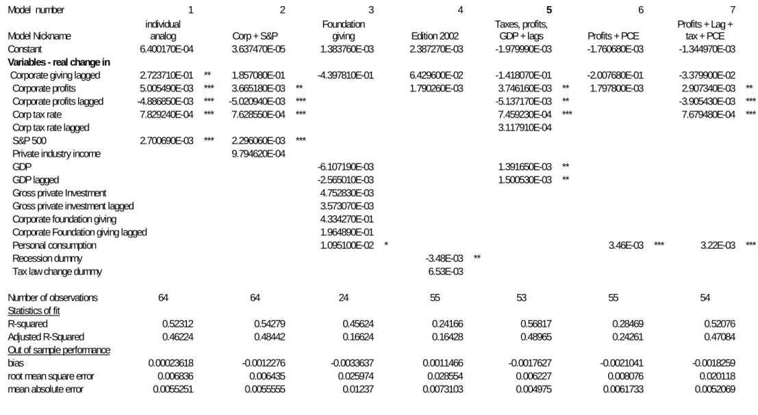
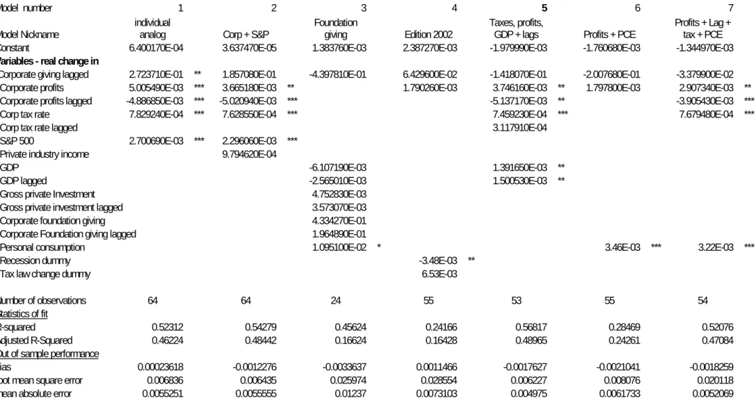
Table 1 presents a comparison of selected models examined in the final phase of our analysis.
Selected competing models are in columns 2 to 8 with the top row indicating model number and the second row indicating the model “nickname.” In the body of the table are coefficient
estimates for the various models which match the variables in the first column. In the lower rows of the table are standard statistics of fit, R-square and adjusted R-square for the OLS regression of equation 2 above. On the lowest rows of the table are out-of-sample bias, root mean square error and mean absolute error based on equation 1 above. The selected models presented in the table were of special interest because it either ranked highly in our selection procedure outlined above (models 2, 5 and 6) or were of interest in their own right because they are natural
analogues to the individual model, (model 1), or they used The Foundation Center’s data, (model 3), or other special reasons.
The table also indicates coefficients that were significant according to standard t-tests at levels of 10, 5 or 1 percent. We emphasize that the t-tests are based on the regression given by equation 2 above. While these statistics are often used to inform on whether a particular variable belongs in a model, this procedure is only appropriate for in-sample regressions. In other words, we are not seeking to fit equation 2, the process generating changes in corporate itemized giving. Rather, we are seeking to establish a model that has shown good out of sample performance (by fitting
3 We chose to use model rankings rather than assign a specific weight to each criterion because a function
combining the criteria would spell out a particular penalty function in our selection. Given there is no real guide as to how RMSE should be compared to MAE for example, we chose to use rankings in a more agnostic approach. In any case, these procedures are only intended to sift though an overwhelming number of models to a handful that can
equation 1) given the informational lags faced by Giving USA in each of its editions. Thus, we do not hesitate in choosing models with seemingly insignificant variables because our emphasis is on the out-of-sample performance of our models.
Figure 3 depicts a graphic showing the bias, root mean square error and mean absolute error of models 1 thru 7. It can be seen that some models had a positive bias while others had a negative bias. Among the selected models, model 1 has the smallest (absolute) bias. Model 5 has the lowest root mean square error and mean absolute error among all the models generated. Figures 4 and 5 show the projections from various model compared with actual corporate giving.
We recommended Model 5 as the forecasting model for corporate itemized giving for Giving USA. Although this model did not exhibit the smallest absolute bias, it ranked best in terms of having the smallest root mean square error and mean absolute error over the period 1986 to 2000 as well as best overall when we added the rank scores across all three criteria.
The parameter estimates of model 5 are largely consistent with economic theory. For example, economic theory would suggest the coefficient for corporate tax rates should be positive- higher tax rates and higher tax deductibility of corporate contributions should lead to higher
contributions. Our model estimates that a one percent increase in corporate tax rates increases corporate contributions by 0.0746 billion in the year in which the change is made and by 0.0206 billion in the following year. An increase in GDP in year t by 1 billion dollars increases
corporate contribution by 1.39 million in year t and by 1.30 million in year t+1. An increase in corporate profits in year t by 1 billion dollars increases corporate contribution by 3.746 million in year t and decreases it by 5.668 in year t+1.4
Another factor that added to the appeal of model 5 over others was what appeared to be the stability of the coefficient estimates. From figure 2, it can be seen that the inner loop executes 15 regressions of equation 2 to compute corporate giving forecasts from 1986 to 2000. The
4 The use of lag operators (covered in most time series texts, e.g. Hamilton (1994)) greatly simplifies the calculation of these dynamics. Using L to denote a lag operation, the forecasting model is
) L 1 /(
] tax . corp ) L (
GDP ) L (
profits . corp ) L (
[
c 2
^ t
7
^ 6
^ t 6
^ 5
^ t 4
^ 3
^ 1
^ t
^ = β + β +β + β +β + β +β −β .
coefficient estimates seemed to change little over the 15 regressions as longer time series were used when compared to other models. Model 5 also has a better in-sample fit when one compares the R-square and adjusted R-square statistic to many of the models analyzed
Finally, it was considered important to choose a model with a relatively precise estimate of the coefficient β2. Note from equation 3b that the estimate for the change in corporate giving in year t, t
^
c , will itself use an estimate for corporate giving in year t-1, t 1
^
c − , from equation 3a. Thus, if lagged corporate giving is to be used in equation 2 to estimate the structural coefficients to changes in corporate giving, then the forecasting equation will be non-linear because equation 3b is non-linear. Specifically, equation 3b is non-linear because the coefficient β2 multiplies all other coefficients in equation 3a. Despite this, the OLS estimation of equation 2 will provide a consistent estimate of all parameters and the multiplication of consistent parameters will itself be consistent.
Our choice of model 5 was guided by a wider set of criteria than the ranking of this model alone.
Other considerations that were considered important were consistency with economic theory, stability of parameter estimates, a high in-sample fit and a relatively precise estimate of the coefficientβ2.
Table 1. Corporate Giving estimating Models 1-7:
Table of coefficients, statistics of fit and out-of-sample performance
Note:- # indicates price deflated differences * p<0.10, ** p<0.05, *** p<0.01
Model number 1 2 3 4 5 6 7
Model Nickname
individual
analog Corp + S&P
Foundation
giving Edition 2002
Taxes, profits,
GDP + lags Profits + PCE
Profits + Lag + tax + PCE Constant 6.400170E-04 3.637470E-05 1.383760E-03 2.387270E-03 -1.979990E-03 -1.760680E-03 -1.344970E-03 Variables - real change in
Corporate giving lagged 2.723710E-01 ** 1.857080E-01 -4.397810E-01 6.429600E-02 -1.418070E-01 -2.007680E-01 -3.379900E-02 Corporate profits 5.005490E-03 *** 3.665180E-03 ** 1.790260E-03 3.746160E-03 ** 1.797800E-03 2.907340E-03 **
Corporate profits lagged -4.886850E-03 *** -5.020940E-03 *** -5.137170E-03 ** -3.905430E-03 ***
Corp tax rate 7.829240E-04 *** 7.628550E-04 *** 7.459230E-04 *** 7.679480E-04 ***
Corp tax rate lagged 3.117910E-04 S&P 500 2.700690E-03 *** 2.296060E-03 ***
Private industry income 9.794620E-04
GDP -6.107190E-03 1.391650E-03 **
GDP lagged -2.565010E-03 1.500530E-03 **
Gross private Investment 4.752830E-03 Gross private investment lagged 3.573070E-03
Corporate foundation giving 4.334270E-01
Corporate Foundation giving lagged 1.964890E-01 Personal consumption 1.095100E-02 * 3.46E-03 *** 3.22E-03 ***
Recession dummy -3.48E-03 **
Tax law change dummy 6.53E-03
Number of observations 64 64 24 55 53 55 54 Statistics of fit
R-squared 0.52312 0.54279 0.45624 0.24166 0.56817 0.28469 0.52076 Adjusted R-Squared 0.46224 0.48442 0.16624 0.16428 0.48965 0.24261 0.47084 Out of sample performance bias 0.00023618 -0.0012276 -0.0033637 0.0011466 -0.0017627 -0.0021041 -0.0018259 root mean square error 0.006836 0.006435 0.025974 0.028554 0.006227 0.008076 0.020118 mean absolute error 0.0055251 0.0055555 0.01237 0.0073103 0.004975 0.0061733 0.0052069
Figure 4
Projections of models 3, 4 and 7 against actual corporate giving
0 2 4 6 8 10 12 14
1988 1989 1990 1991 1992 1993 1994 1995 1996 1997 1998 1999 2000 2001 2002 year
billions Model 3
Model 4 Model 7 Actual
Figure 5
Projections of models 1, 2, 5 and 6 against actual corporate giving
0 2 4 6 8 10 12 14
1988 1989 1990 1991 1992 1993 1994 1995 1996 1997 1998 1999 2000 2001 2002 year
billions
Model 1 Model 2 Model 5 Model 6 Actual
Conclusion
The problem of deriving an estimate for corporate giving for each edition of Giving USA is truly an out-of-sample forecasting problem. Following the impetus of making
methodological improvements to all components of Giving USA, a systematic evaluation of a very large number of corporate giving forecasting models was performed.
Our procedure was largely driven by the number of variables suggested by the Giving USA Advisory Council on Methodology. Unlike the case of the individual giving model reported in Deb, et al which had a comparatively smaller set of models to test, what was required for the development of the corporate giving model was a ready means of both generating large numbers of models and storing performance criteria for each model generated.
Using a batch computer program that rotated in all the suggested variables and mean error, root mean squared error and mean absolute error as performance criteria, a vast number of models were explored and ranked relatively easily. We emphasize that the rank performance of models on our three performance criteria was not the sole factor in our final choice to recommend model 5. In drawing comparisons between special models of interest, parameter stability and concordance with economic theory were considered as important as outright minimization of out-of-sample errors.
But to make detailed evaluations of anything more that a dozen or so models becomes unwieldy and impractical. Our procedure of generating models and sifting them by rank performance allowed us to concentrate on some of the best ranked models and compare those to other models of special interest. Our extensive search gives us confidence that the forecasting model chosen for corporate giving in Giving USA is among the best of all possible forecasting models.
Appendix
Autocorrelation Function of: RCORGIV
-1.00 -0.60 -0.20 0.20 0.60 1.00 |-+---+---+----0----+---+---+-|
1 | + | + R | 0.89432
2 | + | + R | 0.81875
3 | + | + R | 0.74432
4 | + | + R | 0.68092
5 | + | R | 0.61805
6 | + | R + | 0.57928
7 | + | R + | 0.54354
8 | + | R + | 0.52031
9 | + | R + | 0.50559
10 | + | R + | 0.48294
11 | + | R + | 0.44570
12 | + | R + | 0.40209
13 | + | R + | 0.35369
14 | + | R + | 0.29238
15 | + | R + | 0.24647
16 | + | R + | 0.20961
17 | + | R + | 0.16288
18 | + | R + | 0.13423
19 | + | R + | 0.11153
20 | + | R + | 0.086549
|-+---+---+----0----+---+---+-|
-1.00 -0.60 -0.20 0.20 0.60 1.00 Partial Autocorrelation Function of: RCORGIV
-1.00 -0.60 -0.20 0.20 0.60 1.00 |-+---+---+----0----+---+---+-|
1 | + | + R | 0.97706
2 | +R | + | - 0.19567
3 | + R| + | - 0.049540
4 | + R + | 0.0081815
5 | + R | + | - 0.12093
6 | + | R + | 0.14360
7 | + R | + | - 0.088190
8 | + R| + | - 0.042665
9 | + | R + | 0.068534
10 | + R | + | - 0.12356
|-+---+---+----0----+---+---+-|
-1.00 -0.60 -0.20 0.20 0.60 1.00 Autocorrelation Function of: (1-B) RCORGIV
-1.00 -0.60 -0.20 0.20 0.60 1.00 |-+---+---+----0----+---+---+-|
1 | + | R + | 0.092429
2 | + R + | - 0.013251
3 | + R | + | - 0.079352
4 | + |R + | 0.034517
5 | + R | + | - 0.16082
6 | + R + | - 0.010937
7 | + R + | 0.017632
8 | + R | + | - 0.069596
9 | + |R + | 0.040331
10 | + |R + | 0.048681
11 | + R | + | - 0.087208
12 | + R | + | - 0.10909
13 | + |R + | 0.058201
14 | + R + | 0.019449
15 | + |R + | 0.021413
16 | + | R + | 0.14482
17 | + | R + | 0.078223
18 | + R| + | - 0.021519
19 | + R | + | - 0.078804
20 | + | R + | 0.089464
|-+---+---+----0----+---+---+-|
-1.00 -0.60 -0.20 0.20 0.60 1.00 Partial Autocorrelation Function of: (1-B) RCORGIV
-1.00 -0.60 -0.20 0.20 0.60 1.00 |-+---+---+----0----+---+---+-|
1 | + | R + | 0.10477
2 | + R| + | - 0.027081
3 | + R | + | - 0.080933
4 | + |R + | 0.058117
5 | +R | + | - 0.20119
6 | + |R + | 0.026815
7 | + R + | - 0.0011836
8 | + R | + | - 0.12632
9 | + | R + | 0.069605
10 | + R + | - 0.0088313
|-+---+---+----0----+---+---+-|
-1.00 -0.60 -0.20 0.20 0.60 1.00
2
Autocorrelation Function of: (1-B) RCORGIV
-1.00 -0.60 -0.20 0.20 0.60 1.00 |-+---+---+----0----+---+---+-|
1 | R + | + | - 0.36360
2 | + R| + | - 0.051936
3 | + R | + | - 0.080238
4 | + | R + | 0.13287
5 | + R | + | - 0.14553
6 | + R + | 0.014001
7 | + | R + | 0.069658
8 | + R| + | - 0.045198
9 | + | R + | 0.084691
10 | + | R + | 0.076607
11 | + R | + | - 0.064156
12 | + R | + | - 0.098364
13 | + R + | 0.0061628
14 | + R + | 0.013690
15 | + R | + | - 0.093002
16 | + | R + | 0.086804
17 | + | R + | 0.061352
18 | + R + | 0.014829
19 | + R | + | - 0.12375
20 | + |R + | 0.034454
|-+---+---+----0----+---+---+-|
-1.00 -0.60 -0.20 0.20 0.60 1.00
2
Partial Autocorrelation Function of: (1-B) RCORGIV
-1.00 -0.60 -0.20 0.20 0.60 1.00 |-+---+---+----0----+---+---+-|
1 | R + | + | - 0.39041
2 | R | + | - 0.24562
3 | R+ | + | - 0.28677
4 | + R| + | - 0.029886
5 | R | + | - 0.22522
6 | + R | + | - 0.16468
7 | + R| + | - 0.046818
8 | + R | + | -
9 | + R| + | - 0.022843
10 | + | R + | 0.13238
|-+---+---+----0----+---+---+-|
-1.00 -0.60 -0.20 0.20 0.60 1.00 Current sample: 38 to 62
References
Boatsman, J. and Gupta, S. (1996). Taxes and corporate charity: empirical evidence from microlevel panel data. National Tax Journal, 49, 2, 193-214. citation page 193.
Brudney, V. (2002). Corporate charitable giving. University of Chicago Law Review, 69, 3, 1191-1218.
Deb, P. Wilhelm, M., Rooney, P., and Brown, M. 2003, “Estimating individual charitable giving,” Nonprofit and Voluntary Sector Quarterly, forthcoming (December 2003).
Giving USA, Ann Kaplan, ed., editions 1995-2000 (AAFRC Trust for Philanthropy: New York)
Giving USA, Center on Philanthropy, ed., editions 2001-2003 (AAFRC Trust for Philanthropy: Indianapolis).
Greene, W. H. (2000). Econometric Analysis (Fourth edition). Upper Saddle River, NJ:
Prentice-Hall.
Hamilton, J. D. (1994). Time Series Analysis. Princeton University Press, Princeton, New Jersey.
Himmelstein, J.L. (1997). Looking Good & Doing Good: Corporate Philanthropy and Corporate Power (Indiana University Pres: Bloomington)
Johnson, W. and Johnson, O. (1970). The income elasticity of corporate philanthropy:
comment. Journal of Finance, 26, 1, 149-52.
Kinane, Pamela, 2003, personal correspondence with Melissa Brown, managing editor of Giving USA, by e-mail, June 25, 2003.
Levy, Reynold (1999) Give and Take: A Candid Account of Corporate Philanthropy (Harvard Business School Press: Cambridge, MA)
Lowenstein, Roger, 2003 “Nothing charitable about giving in,” The Washington Post, July 20, 2003, Outlook section, Pg. B3.
Mark OKeefe, 2003, Corporate giving prospers : Philanthropy remains business goal even in economic downturn, Seattle Times, June 24, 2003, page D3.
Muirhead, S. (2002) Corporate Charitable Contributions, 2001. (Conference Board: New York)
Navarro, P. (1988). Why do corporations give to charity? Journal of Business. 61,1, 65- 93.
Nelson, R. (1970). Economic Factors in the Growth of Corporate Giving, National Bureau of Economic Research, New York. 1970.
O’Neill, M. (2002). Nonprofit Nation: A New Look at the Third America, (Jossey-Bass:
San Francisco), p. 195.
Renz, L., 2002. Giving in the Aftermath of 9/11: An Update on Corporate and Foundation Response, (Foundation Center: New York)
Salmon, J. (2003, July 6). As companies shave aid, nonprofits suffer the sting, The Washington Post, p. A 01.
Schwartz, R. (1968). Corporate philanthropic contributions. Journal of Finance, XXIII, 3, 479-497.
Seifert, B., Morris, S., and Bartkus, B. (YEAR). “Comparing big givers and small givers:
Financial correlates of corporate philanthropy, Journal of Business Ethics, 45, 3, 195-211.
Seifert, B., Morris, S., Bartkus, B. (2003). Comparing big givers and small givers:
Financial correlates of corporate philanthropy. Journal of Business Ethics, 45, 195-211.
Shannon, J.P. (1991). Preface. In J.P. Shannon (ed.) The Corporate Contributions Handbook (Jossey-Bass: San Francisco, CA)
Strom, S. (2003, June 23). Gifts to Charity in 2002 Stayed Unexpectedly High. The New York Times, p. A14.
Wallack, T. (2003, April 20). S.F. arts groups weather donation slowdown, San Francisco Chronicle, p. A 20.
Weitzman, M., Jalandoni, N., Lampkin, L., and Pollak, T. (2002). The New Nonprofit Almanac & Desk Reference (Jossey-Bass: San Francisco), p. 59.
Wooldridge, J.M. (2000). Introductory Econometrics. Cincinnati, OH: South-Western College Publishing