The third generation eye tracker was used for most of the eye tracking research on which the first edition of this book was based. The fourth part of the book covers a number of interesting and challenging eye tracking applications.
Introduction to the Human Visual System (HVS)
Visual Attention
Visual Attention: A Historical Review
- Von Helmholtz’s “Where”
- James’ “What”
- Gibson’s “How”
- Broadbent’s “Selective Filter”
- Deutsch and Deutsch’s “Importance Weightings”
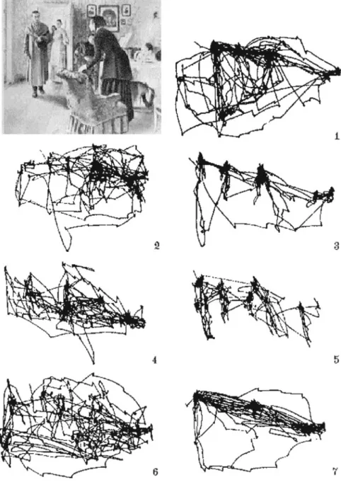
- Yarbus and Noton and Stark’s “Scanpaths”
- Posner’s “Spotlight”
- Treisman’s “Glue”
- Kosslyn’s “Window”
James defined attention primarily in terms of the "what," or identity, meaning, or expectation associated with the focus of attention. In terms of the "what" and the "where," it seems likely that the "what" pertains to serial foveal vision.
Visual Attention and Eye Movements
The novelty of the attention window is its ability to be adjusted incrementally; that is, the window is scalable. That is, through psychophysics we can measure the perceptual power of the human visual system quite well.
Summary and Further Reading
An eye tracker can only track the overt movements of the eyes, but it cannot track the covert movement of visual attention. Thus, in all eye tracking work, a tacit but very important assumption is usually accepted: we assume that attention is linked to foveal gaze direction, but we recognize that this may not always be the case.
Neurological Substrate of the HVS
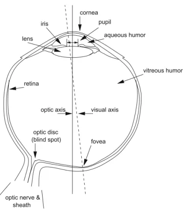
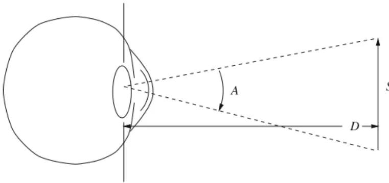
- The Eye
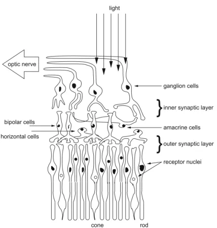
- The Retina
- The Outer Layer
- The Inner Nuclear Layer
- The Ganglion Layer
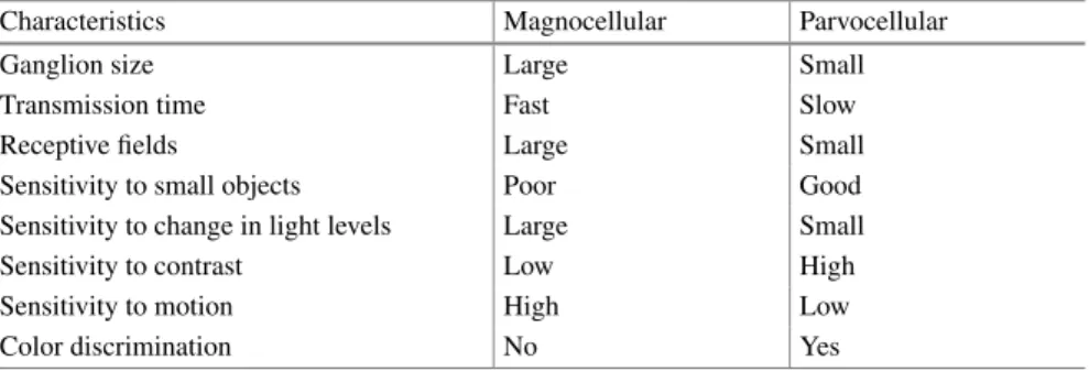
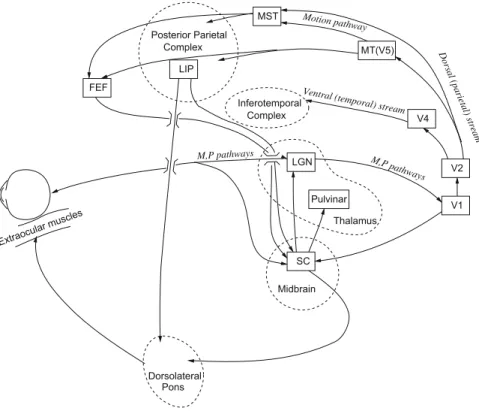
- The Optic Tract and M/P Visual Channels
- The Occipital Cortex and Beyond
- Motion-Sensitive Single-Cell Physiology
- Summary and Further Reading
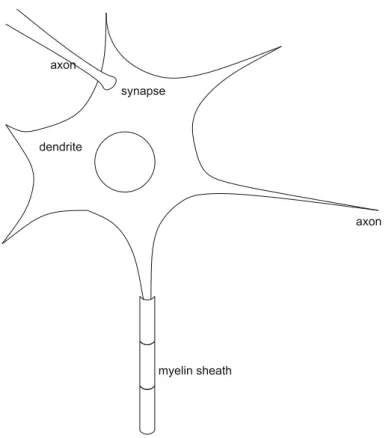
Unmyelinated ganglion cell axons converge on the optic disc (a dark myelin sheath would block light). An object in the visual field stimulates only a small fraction of cells in its receptive field (Hubel 1988).
Visual Psychophysics
- Spatial Vision
- Temporal Vision
- Perception of Motion in the Visual Periphery
- Sensitivity to Direction of Motion in the Visual PeripheryPeriphery
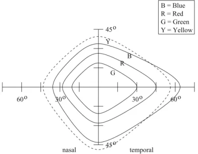
- Color Vision
- Implications for Attentional Design of Visual Displays
- Summary and Further Reading
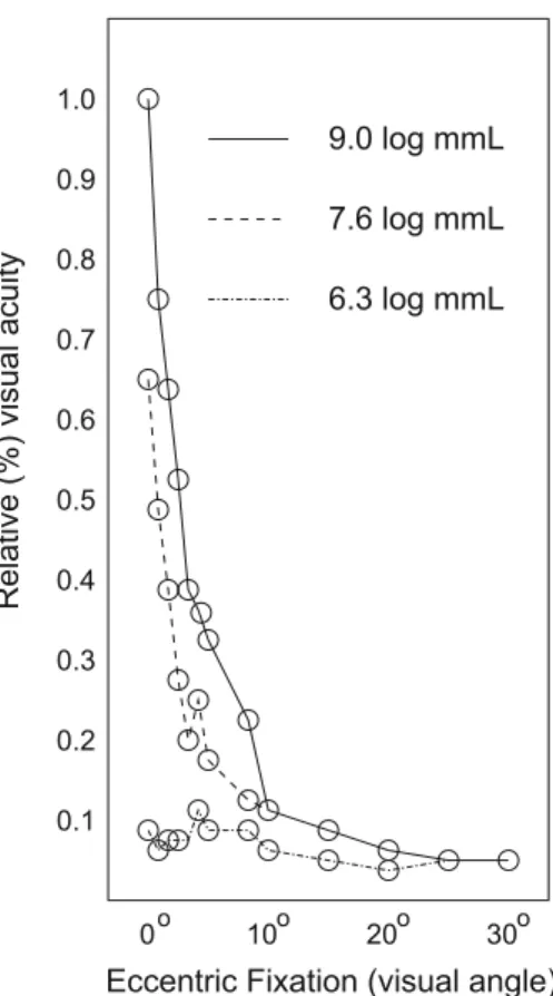
This requirement is a direct consequence of the high density of cones and parvocellular ganglion cells in the fovea. Contrast sensitivity should be high in the periphery, corresponding to the sensitivity of the magnocellular ganglion cells found mainly outside the fovea.
Taxonomy and Models of Eye Movements
- The Extraocular Muscles and the Oculomotor Plant
- Saccades
- Smooth Pursuits
- Fixations (Microsaccades, Drift, and Tremor)
- Nystagmus
- Implications for Eye Movement Analysis
- Summary and Further Reading
The feedback-like circuits are mainly used in the types of eye movements that require stabilization of the eye. Vestibular nystagmus is a similar type of eye movement that compensates for head movement. This conference series has recently been revived in the form of the (currently biannual) Eye Tracking Research & Applications (ETRA) conference.
Eye Tracking Systems
Eye Tracking Techniques
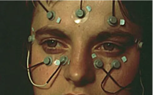
- Electro-OculoGraphy (EOG)
- Scleral Contact Lens/Search Coil
- Video-Based Combined Pupil/Corneal Reflection
- Classifying Eye Trackers in “Mocap” Terminology
- Summary and Further Reading
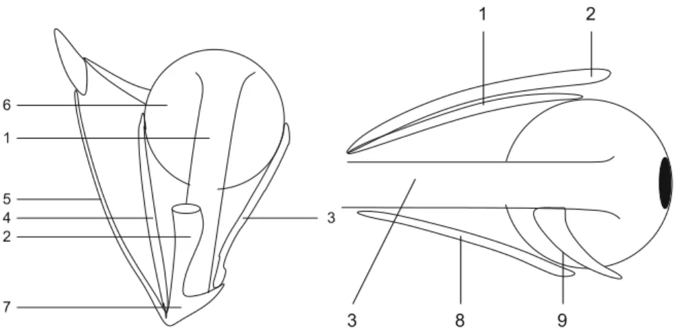
One of the most accurate eye movement measurement methods involves attaching a mechanical or optical reference object mounted on a contact lens, which is then worn directly on the eye. The corneal reflectance of the light source (typically infrared) is measured relative to the location of the pupil center. Due to the construction of the eye, four Purkinje reflexes are formed, as shown in Fig.5.7.
Head-Mounted System Hardware Installation
- Integration Issues and Requirements
- System Installation
- Lessons Learned from the Installation at Clemson
- Summary and Further Reading
The ability of the eye tracker to provide precise control of the cursor over its calibration stimulus (crosshair or other symbol). The ability of the eye tracker to communicate its mode of operation to the host along with information about the eyes and gaze points. However, after inserting the HMD into the video circuit, the eye tracker would not work.
Head-Mounted System Software Development
Mapping Eye Tracker Screen Coordinates
- Mapping Screen Coordinates to the 3D Viewing FrustumFrustum
- Mapping Screen Coordinates to the 2D Image
- Measuring Eye Tracker Screen Coordinate Extents
Figure 7.1 shows the dimensions of the eye tracker screen (left) and the dimensions of the vision block (right). The above coordinate mapping procedures assume that the eye tracker coordinates are in the range[0,511]. To see the extent of the application window in the eye tracker's reference frame, simply move the cursor to the corners of the application window.
Mapping Flock of Birds Tracker Coordinates
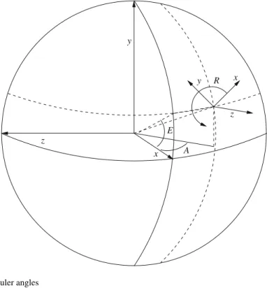
- Obtaining the Transformed View Vector
- Obtaining the Transformed up Vector
- Transforming an Arbitrary Vector
To calculate the transformed up vector u′, we assume that the initial up vector is u=(0,1,0) (looking along the y-axis), and apply the compound transformation (in homogeneous coordinates): . cosRcosA+sinRsinEsinA sinRcosE −cosRsinA+sinRsinEcosA0. By inspection of the Bird matrix F, the transformed vector is obtained simply by selecting the appropriate items in the matrix; i.e.,. 7.11) Because of our setup in the lab, the z-axis is on the opposite side of the Bird transmitter (behind the Bird decal on the transmitter). Note that the negation of the z component of the transformed image vector makes no difference because the term is a product of cosine.
7.3 3D Gaze Point Calculation
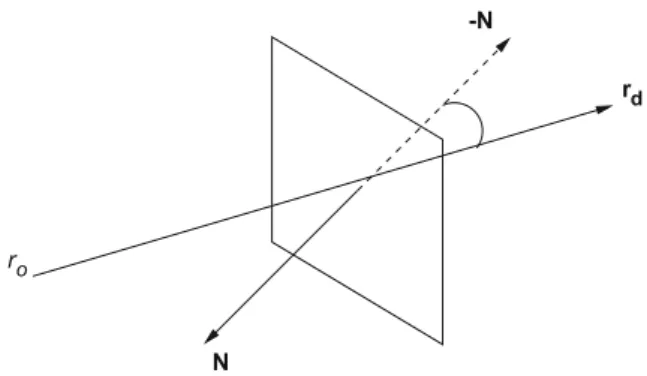
- Parametric Ray Representation of Gaze Direction
- Virtual Gaze Intersection Point Coordinates
- Ray/Plane Intersection
- Point-in-Polygon Problem
- Data Representation and Storage
- Summary and Further Reading
The computation of an intersection between a ray and all polygons in the scene is usually obtained through a parametric representation of the ray; e.g.,. Note that the above only gives the intersection of the radius and the (infinite!) plane defined by the normal of the polygon. One of the easiest methods of encoding this information is in the data file name itself (at least on file systems that allow long file names).
Head-Mounted System Calibration
Software Implementation
This routine is sensitive to the eye tracker's three possible states: RUN, RESET, and CALIBRATE. This facilitates the initial alignment of the application window with the eye tracker's initial reticle positioning. Reading data from the eye tracker (and head tracker, if one is in use).
Ancillary Calibration Procedures
- Internal 2D Calibration
- Internal 3D Calibration
Hence, internal calibration is used to check the accuracy of the eye tracker before and after the stimulus display, to check if the instrument slips. The eye is judged stable once the eye tracker has repositioned the eye in the center of the camera frame. To quantify this correspondence, a one-way ANOVA can be performed on the means of the readings before and after looking at the mean error.
Summary and Further Reading
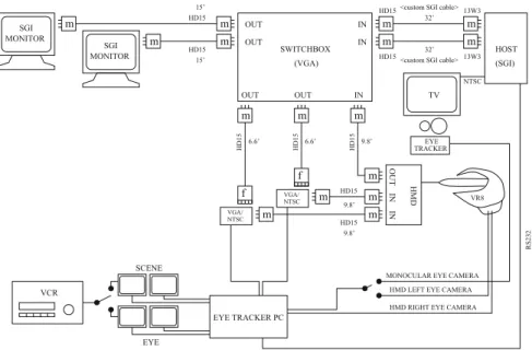
This chapter focuses on the installation of a fourth-generation table-mounted eye tracker (see the analog video or third-generation table-mounted eye tracker discussed in Chapter 6). A table-mounted eye tracker may look indistinguishable from a regular flat panel display, and that's on purpose. The two-head installation at Clemson University, on which this and the remaining chapters of the table-mounted system are based, is shown in Fig.9.1.
Integration Issues and Requirements
The ability of the eye tracker to transmit its operating mode along with gaze (x,y) coordinates. Transferring control to the software allows the client application to control the eye tracker from within. Knowledge of the data format that the eye tracker generates as its output (provided by the SDK reference).
System Installation
For diagnostic users of eye tracking technology, Tobii (as well as other manufacturers) has made great strides towards plug-and-play usability. For the triple installation, both the eye tracking server and application client computers should be equipped with dual-headed graphics cards if one also wants to perform diagnostic eye tracking work on the server machine. If a small monitor is not available, then the alternative is to share the eye tracking display between both server and client computers via a KVM or Keyboard-Video-Mouse switch.
Lessons Learned from the Installation at Clemson
Although the three-head setup may be somewhat redundant, it ultimately needs to interact with the operating system the eye tracking server is running on, and therefore, it needs to be able to connect the display to the eye tracking server. The KVM switch is removed from the schematic in Fig.9.2, as are the keyboard and mouse. The firmware update made available by the KVM switch manufacturer eventually alleviated the problem, but installing the firmware itself was more annoying.
Summary and Further Reading
From the typical installation of one or two eye trackers in a laboratory, a recent trend is to develop larger eye laboratories or classrooms, e.g. see the Clemson installation shown in Figure 9.3. Collecting data from multiple eye trackers simultaneously opens up new possibilities for interesting research and applications. Although specific to the Tobii eye tracker, most eye trackers are expected to contain similar functionality, such as connection to the eye tracker (TCP/IP or serial port), calibration and data streaming.
Linux Tobii Client Application Program Interface
The interval argument specifies an interval in milliseconds when the callback function is called; if set to 0, the callback will never be called for a timer reason (but will be called when new gaze data is available). Set the interval parameter to something other than 0 and the callback function will be called with ETet_CallbackReason set to TET_CALLBACK_TIMER and pDataset set to NULL. Using a different address to connect to localhost introduces an unnecessary error in the timestamps.
A Simple OpenGL/GLUT GUI Example
Listing 10.14 shows the calibration pseudocode. Tet_CalibClearis called once per calibration to clear all calibration information on the eye tracking server. Note that Tet_Starsis is a blocking function and transfers control to the eye tracking client callback, in this case the gazeDataReceiver function, shown in Listing 10.17. Listing 10.17 consumes view data as it becomes available and copies the data into the shared state object.
Caveats
Once this is achieved, the successive coordinates of the calibration points are sent to the eye tracking server one after the other. If it is detected that the operating mode has transitioned to stop (idle) mode, a call to Tet_Stopis is made, returning control to the point where Tet_Start was called. That is, concurrency and synchronization may still be present, but may be transparent to the programmer.
Summary and Further Reading
In some ways, the complexity of calibration has shifted from the user to the application developer. For example, Tobii includes a track status window that displays the location of the user's eyes from the camera's point of view. This is clearly a design decision and depends on the nature of the application being developed.
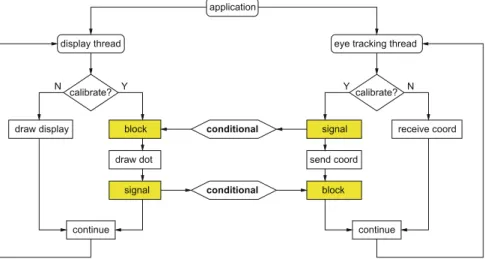
Software Implementation
The intuitive blocking strategy blocks the ET thread while the GUI thread pulls the calibration point. At this point the ET thread blocks itself and waits for the GUI thread to finish drawing the calibration point. If the next coordinates in the sequence were available, the GUI thread would go before the ET thread.
Summary and Further Reading
Using an Open Source Application Program Interface
- API Implementation and XML Format
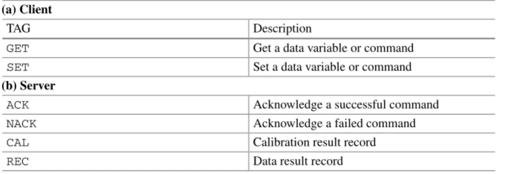
- Client/Server Communication
- Server Configuration
- API Extensions
- Interactive Client Example Using Python
- Using Gazepoint’s Built-in Calibration
- Using Gazepoint’s Custom Calibration Capabilities
- Summary and Further Reading
The Gazepoint API described here corresponds to version 2.0 of the open source interface, identified by the VER_ID variable. Some code snippets are provided here to give an example of how the client/server communication is set up. The timing between points can be used to produce a pleasant animation of the calibration point between stationary targets.
Eye Movement Analysis
- Signal Denoising
- Dwell-Time Fixation Detection
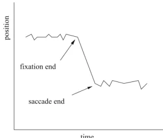
- Velocity-Based Saccade Detection
- Eye Movement Analysis in Three Dimensions
- Parameter Estimation
- Fixation Grouping
- Eye Movement Data Mirroring
- Summary and Further Reading
To eliminate excessive noise in the eye movement signal, the two-tap FIR filter can be replaced by a five-tap FIR filter, as shown in Figure 13.7a. The acceleration filter is shown in Figure 13.7b and is convolved with eye movement velocity data obtained through a two-tap or five-tap velocity filter. The acceleration is obtained by post-convolution of the velocity θ˙i with the acceleration filter gj shown in Figure 13.7b.
Advanced Eye Movement Analysis
- Signal Denoising
- Velocity-Based Saccade Detection
- Microsaccade Detection
- Validation: Computing Accuracy, Precision, and Refittingand Refitting
- Binocular Eye Movement Analysis: Vergence
- Ambient/Focal Eye Movement Analysis
- Transition Entropy Analysis
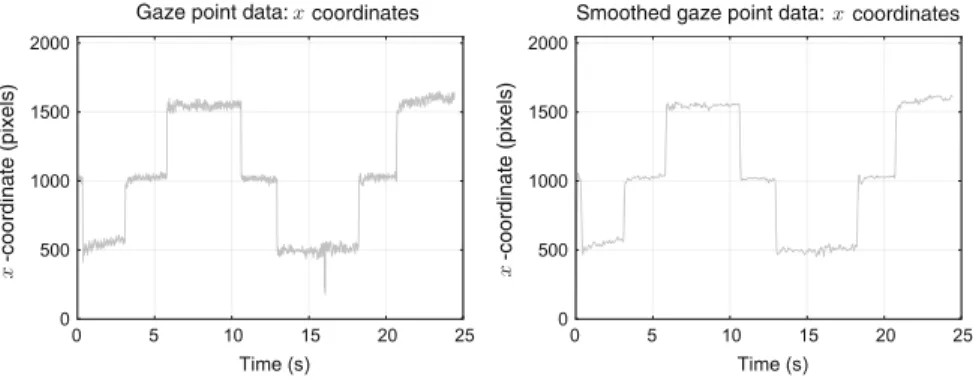
An example of the effect of the Butterworth filter on the x-coordinate of eye movement data is shown in Fig. 14.1, with 2D eye movement data depicted in Fig. 14.2. A multiple of the standard deviation of the velocity distribution is used as the detection threshold (Engbert 2006). As used in the 9-point calibration described by Morimoto and Mimica (2005), define (si x,si y) as the ith calibration point and (x¯i,y¯i) as the centroid of the observed points closest to the calibration point.