forecasting short-run ﬂuctuations - Spada UNS

(1)

Yunastiti Purwaningsih

(2)

(3)

• Economists call these short-run ﬂuctuations in output and employment the business cycle .

• Recessions are actually as irregula r as they are

common. Sometimes they occur close together,

while at other times they are much farther apart.

(4)

• Ekspansi atau ledakan : periode dalam siklus bisnis dari lembah naik ke puncak, dimana pada periode itu output dan

kesempatan kerja meningkat.

• Kontraksi, resesi, atau

penurunan : periode dari puncak turun ke lembah, dimana selama periode itu output dan kesempatan kerja menurun.

Kegiatan perekonomian dalam memproduksi barang dan jasa, naik turun mengikuti siklus bisnis

Kegiatan perekonomian dalam

memproduksi barang dan jasa  GDP (Gross Domestic Product) = PDB (Produk Domestik Bruto)

4

Economists call these short-run ﬂuctuations in output and employment the business cycle

(5)

Kegiatan perekonomian dalam memproduksi barang dan jasa, naik turun mengikuti siklus bisnis

Kegiatan perekonomian dalam

memproduksi barang dan jasa  GDP (Gross Domestic Product) = PDB (Produk Domestik Bruto)

5

Output gap: positif atau negatif

(6)

• For example:

– The United States fell into recession in 1982, only two years after the previous downturn.

– By the end of that year, the unemployment rate had

reached 10.8 percent—the highest level since the Great Depression of the 1930s.

– But after the 1982 recession, it was eight years before the economy experienced another one.

(7)

Contoh: Indonesia tahun 1998

Pertumbuhan Ekonomi

(8)

(9)

9

PDB dan komponennya

(10)

(11)

PDB dan komponennya

(12)

Real GDP Growth in the United States

(13)

Growth in Consumption and Investment When the economy heads

into a recession, growth in real consumption and investment

spending both decline. Investment spending, shown in panel (b), is considerably more volatile than consumption spending, shown in panel (a). The shaded areas

represent periods of recession.

Source: U.S. Department of Commerce.

PDB dan komponennya

(14)

PDB dan komponennya

(15)

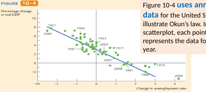
This negative relationship between unemployment and GDP is called Okun’s law, after Arthur Okun, the economist who ﬁrst studied it.

Tingkat Pengangguran dan Hukum Okun

Figure 10-4 uses annual data for the United States to illustrate Okun’s law. In this scatterplot, each point

represents the data for one year.

(16)

Indonesia

(17)

This negative relationship between unemployment and GDP is called Okun’s law, after Arthur Okun, the economist who ﬁrst studied it

if the unemployment rate remains the same, real GDP grows by about 3

percent; this normal growth in the production of goods and services is due to growth in the labor force, capital accumulation, and technological progress.

Tingkat Pengangguran dan Hukum Okun

(18)

This negative relationship between unemployment and GDP is called Okun’s law, after Arthur Okun, the economist who ﬁrst studied it

In this case, Okun’s law says that GDP would fall by 1 percent, indicating that the economy is in a recession.

The declines in the production of goods and services that occur during recessions are always associated with increases in joblessness.

Tingkat Pengangguran dan Hukum Okun

(19)

Leading Economic Indicators

• Many economists, particularly those working in business and government, are engaged in the task of forecasting short-run ﬂuctuations in the economy.

• Business economists are interested in forecasting to help their

companies plan for changes in the economic environment.

• Government economists are interested in forecasting for two reasons. – First, the economic environment affects the government; for example, the

state of the economy inﬂuences how much tax revenue the government collects.

– Second, the government can affect the economy through its use of monetary and ﬁscal policy.

• Economic forecasts are, therefore, an input into policy planning.

• One way that economists arrive at their forecasts is by looking at leading indicators, which are variables that tend to ﬂuctuate in advance of the

overall economy.

• Forecasts can differ in part because economists hold varying opinions about which leading indicators are most reliable.

(20)

Leading Economic Indicators

The index of leading economic indicators^.

This index includes ten data series that are often used to forecast changes in economic activity about six to nine months into the future. Here is a list of the series:

(21)

Leading Economic Indicators

The index of leading economic indicators^.

1. Rata-rata produksi per pekerja per minggu di industri manufaktur 2. Rata-rata klaim asuransi pengangguran per minggu

3. Order baru untuk barang konsumsi dan bahan baku, yang disesuaikan dengan inflasi

4. Kinerja vendor, mengukur jumlah perusahaan yang menerima kiriman yang lambat dari supplier

5. Order baru untuk barang modal (bukan untuk pertahanan/militer) 6. Isu ijin pembangunan gedung baru

7. Indeks harga saham

8. Jumlah unag beredar dalam arti luas (M2), yang disesuaikan dengan inflasi

9. Spread suku bunga : spread hasil saham 10 tahun dan tagihan obligasi 3 bulan

10. Indeks ekspektasi konsumsi

(22)

Leading Economic Indicators

INDONESIA

(23)

• Long run:

Prices are ﬂexible, respond to changes in supply or demand

• Short run:

many prices are “sticky” at some predetermined level

The economy behaves much

differently when prices are sticky.

(24)

In Classical Macroeconomic Theory :

(what we studied in chapters 3-8)

• Output is determined by the supply side:

– supplies of capital, labor – technology

• Changes in demand for goods & services (C, I, G ) only affect prices, not quantities.

• Complete price ﬂexibility is a crucial assumption,

• So classical theory applies in the long run.

(25)

When prices are sticky

…output and employment also depend on demand for goods &

services, which is affected by:

 ﬁscal policy (G and T)

 monetary policy (M)

 other factors, like exogenous changes

in C or I.

Variabel Kebijakan:

• Pemerintah: G dan T

• Bank Sentral (BS): M Variabel Eksogen:

• Rumah Tangga: C

• Perusahaan: I

(26)

The model of aggregate demand and supply

• the paradigm that most mainstream economists

& policymakers use to think about economic

ﬂuctuations and policies to stabilize the economy

• shows how the price level and aggregate output are determined.

• shows how the economy’s behavior is different

in the short run and long run.

(27)

• The aggregate demand (AD) curve shows the

relationship between the price level and the quantity of output demanded.

• For this chapter’s intro to the AD/AS model,

we use a simple theory of aggregate demand based on the Quantity Theory of Money.

• Chapters 10-12 develop the theory of aggregate

demand in more detail.

(28)

The Quantity Equation as Aggregate Demand

• From Chapter 4, recall the quantity equation M V = P Y

and the money demand function it implies:

(M/P )

^d

= k Y where V = 1/k = velocity.

• For given values of M and V, these equations

imply an inverse relationship between P and Y:

(29)

An increase in the price level causes a fall in real money

balances (M/P ), causing a decrease in the demand for goods &

services: P  (M/P) ↓  D for goods & services↓  Y ↓

(30)

M V = P Y

The money supply M and the velocity of money V determine the nominal value of output PY.

Once PY is ﬁxed, if P goes up, Y must go down.

M V

^tetap

= P  Y ↓

2 1

3

P1

P2

Y2 Y1

1

2

(31)

(32)

• M ↓  PY ↓ dengan P

tertentu  Y ↓

• M ↓  geser AD kekiri

P1

Y2 Y1

(33)

• M   PY  dengan P

tertentu  Y 

• M   geser AD kekanan

P1

Y1 Y2

(34)

• Recall from chapter 3:

In the long run, output is determined by factor supplies and technology

is the full-employment or natural level of output, the level of output at which the economy’s resources are fully employed.

“Full employment” means that

unemployment equals its natural rate.

Aggregate Supply in the Long Run

 ( , ) Y F K L

Y

(35)

• Recall from chapter 3:

In the long run, output is determined by factor supplies and technology

 Full-employment output does not depend on the price level,

so the long run aggregate supply (LRAS) curve is vertical:

 ( , )

Y F K L

(36)

The LRAS curve is vertical at the full- employment level of output (Ybar).

(37)

Shifts in Aggregate Supply in the Long Run

P1

(38)

Shifts in Aggregate Supply in the Long Run

• LRAS dan AD1 A:

P1 dan Ybar

P1

• LRAS dan AD2 B:

P2 dan Ybar

• M   P  dan Y tetap (Ybar)

• M ↓  AD ↓ geser kiri: AD1 ke AD2;

LRAS tetap

(39)

Long-run effects of an increase in M

Y

P

AD₁

AD₂ LRAS

An increase in M shifts the AD curve to the

right.

P₁ P₂

In the long run, this increases the price level…

…but leaves output the same.

A B

• LRAS dan AD1 A: P1 dan Ybar

• M   AD  geser kanan: AD1 ke AD2 ; LRAS tetap

• LRAS dan AD2 B: P2 dan Ybar

• M   P  dan Y tetap (Ybar)

Y

(40)

The SRAS curve is horizontal:

The price level is ﬁxed at a

predetermined level, and ﬁrms sell as much as buyers demand.

P

(41)

Shifts in Aggregate Demand in the Short Run

M   AD  geser kanan: AD1 ke AD2

 SRAS tetap  P tetap  Y  dari Y1 ke Y2

P

(42)

Short-run effects of an increase in M

Y P

AD₁ AD₂

…an increase in aggregate demand…

In the short run when prices are sticky,…

…causes output to rise.

SRAS

Y₂ Y₁

M   AD  geser kanan: AD1 ke AD2

 SRAS tetap  P tetap pada Pbar  Y

 dari Y1 ke Y2

P

(43)

We can summarize our analysis so far as follows:

• Over

long periods

^{of time,}

prices are ﬂexible,

^the

aggregate supply curve is vertical

, and

changes in aggregate demand affect the price level but not output

.

• Over

short periods

^{of time,}

prices are sticky

^{, the}

aggregate supply curve is ﬂat

^{, and}

changes in

aggregate demand do affect the economy’s

output of goods and services

^.

(44)

We can summarize our analysis so far as follows:

• Over long periods of time, prices are ﬂexible, the aggregate supply curve is vertical, and changes in aggregate demand affect the price level but not output.

• Over short periods of time,

prices are sticky, the aggregate supply curve is ﬂat, and changes in aggregate demand do affect the economy’s output of goods and services.

Jangka Panjang:

P fleksibel.

AS vertikal, ∆AD

 ∆P; Y tetap Jangka Pendek:

P tetap.

AS horinsontal,

∆AD  P tetap; ∆Y

(45)

P1 A

(46)

P

Pada titik A: M ↓  AD ↓ geser kiri: AD1 ke AD2  AD2 dan SRAS  titik B:

P tetap pada P1 dan Y ↓ dari Ybar ke Y1 (Y1<Ybar);

AD2 dan LRAS 

kelebihan AS  P turun sampai pada tingkat Y bar

 titik C: P2 dan Y bar

Y1 P1

P2

(47)

The SR & LR effects of  M > 0

Y P

AD₁ AD₂ LRAS

SRAS P₂

Y₂ A = initial

equilibrium

A

B B = new short-run C

eq’m after Fed increases M

C = long-run equilibrium

M Pada titik A:

……… titik B:

………  titik C: P2 dan Ybar

Y

P

(48)

• shocks : exogenous changes in aggregate supply or demand.  pergeseran AD dan atau AS

• Shocks temporarily push the economy away from full- employment.  Y menjauh dari Y FE

• An example of a demand shock: exogenous decrease in velocity.  Contoh shock di AD: V ↓

• If the money supply is held constant, then a decrease in V means people will be using their money in fewer

transactions, causing a decrease in demand for goods

and services.  M tetap, V ↓ (transaksi ↓)  AD barang

dan jasa ↓

(49)

• One goal of the model of aggregate supply and aggregate demand is to show

how shocks cause economic

ﬂuctuations

.

• Another goal of the model is to evaluate

how

macroeconomic policy can respond to these shocks

.

• Economists use the term

stabilization policy to refer to policy actions aimed at reducing the severity of

short-run economic ﬂuctuations

.

• Because output and employment ﬂuctuate around their long- run natural levels,

stabilization policy

dampens the

business cycle by

keeping output and employment as

close to their natural levels as possible

^.

(50)

Consider an example of a demand shock: the introduction and expanded availability of

credit cards

.

• Because credit cards are often a more convenient way to

make purchases than using cash, they

reduce the quantity of money that people choose to hold

.

• This reduction in money demand is equivalent to

an

increase in the velocity of money

. When each person holds less money, the money demand parameter k falls.

• This means that

each dollar of money moves from

hand to hand more quickly

, so velocity V (= 1/k) rises

(51)

• If the money supply is held constant, the increase in velocity causes nominal spending to rise and the aggregate demand curve to shift outward.  M tetap, V  (transaksi )  AD barang dan jasa   AD geser kanan

• In the short run, the increase in demand raises the output of the economy—it causes an economic boom. jangka pendek: AD barang dan jasa   perekonomian boom

• At the old prices, ﬁrms now sell more output. Therefore, they hire more workers, ask their existing workers to work longer hours, and make greater use of their factories and equipment.

 Pada P semula: perusahaan menjual banyak output  meningkatkan pengerjaan dengan menambah jam kerja;

menambah pengerjaan mesin dan peralatan.

(52)

• Over time, the high level of aggregate demand pulls up wages and prices. As the price level rises, the quantity of output

demanded declines, and the economy gradually approaches the natural level of production.  sepanjang waktu: AD yang

tinggi  upah (w) dan harga (P); P   jumlah agregat yang diminta ↓  perkeonomian secara perlahan menuju ke tingkat output alamiah (Ybar)

• But during the transition to the higher price level, the

economy’s output is higher than its natural level.  selama transisi ke tingkat harga yang lebih tinggi, Y > Ybar

(53)

P1

Y1

Pada titik A: credit card

 V   AD  geser kanan: AD1 ke AD2  AD2 dan SRAS  titik B:

P tetap pada P1 dan Y  dari Ybar ke Y1

(Y1>Ybar); AD2 dan

LRAS  kelebihan AD  P naik  sampai pada tingkat Y bar  titik C:

P2 dan Ybar

P₂

(54)

Pada titik A: credit card  V   AD  geser kanan: AD1 ke AD2  AD2 dan SRAS  titik B: P tetap pada P1 dan Y  dari Ybar ke Y1 (Y1>Ybar);

AD2 dan LRAS  kelebihan AD  P naik  sampai pada tingkat Y bar

 titik C: P2 dan Ybar

• What can the Fed do to dampen this boom and keep output closer to the natural level?

• The Fed might reduce the money supply to offset the increase in velocity. Offsetting the change in velocity would stabilize aggregate demand.

• Thus, the Fed can reduce or even eliminate the impact of demand shocks on output and employment if it can skillfully control the money supply.

• Whether the Fed in fact has the necessary skill is a more difﬁcult question, which we take up in Chapter 18.

(55)

Pada titik A: credit card  V   AD  geser kanan: AD1 ke AD2  AD2 dan SRAS  titik B: P tetap pada P1 dan Y  dari Ybar ke Y1 (Y1>Ybar); M di ↓ kan  AD ↓ geser kiri: AD2 ke AD1  AD1 dan LRAS-SRAS  titik A: P tetap pada P1 dan Y ↓ dari Y1 ke Ybar

P1

Y1

(56)

LRAS

AD₂

SRAS The effects of a negative demand shock

Y P

AD₁ P₂

Y₂ The shock shifts AD

left, causing output and employment to fall in the short run

B A Over time, prices C

fall and the

economy moves down its demand curve toward full- employment.

Pada titik A:

……… titik B:

………  titik C: P2 dan Ybar

P

Y

(57)

Over time, prices gradually become “unstuck.”

When they do, will they rise or fall?

rise fall

remain constant In the short-run

equilibrium, if then over time, the price level will

This adjustment of prices is what moves the economy to its long-run equilibrium.

Y  Y

Y  Y

Y  Y

(58)

Cost   shock AS  P   shock P

(Favorable supply shocks lower costs and prices)

(59)

• Pada titik A: AD dan SRAS1 P1 dan

Ybar

• SRAS ↓ dari SRAS1 ke SRAS2

• SRAS2 dan AD: titik B: P  dari P1 ke P2 dan Y ↓ dari Ybar ke Y1 (Y1<Ybar)

• SRAS ↓  P  dan Y

↓  stagflasi

P1 P2

Y1

SRAS ↓ karena ?

(60)

SRAS₁

Y P

AD LRAS

Y₂ The oil price shock

shifts SRAS up,

causing output and employment to fall.

A In absence of B

further price

shocks, prices will fall over time and economy moves back toward full employment.

SRAS₂

CASE STUDY AS: The 1970s oil shocks

1 A

P

Y

P

2

(61)

• Early 1970s: OPEC coordinates a reduction in the supply of oil.

• Oil prices rose 11% in 1973 68% in 1974 16% in 1975

• Such sharp oil price increases are supply shocks because they signiﬁcantly impact production costs and prices.

CASE STUDY AS: The 1970s oil shocks

(62)

Stabilization policy

• def: policy actions aimed at reducing the severity of short-run economic ﬂuctuations.

• Example: Using monetary policy to combat the

effects of adverse supply shocks:

(63)

Stabilization policy

with monetary policy

P1 P2

• Pada titik A: AD dan SRAS1 P1 dan Ybar

• SRAS ↓ dari

SRAS1 ke SRAS2

• M di  kan  AD

 geser kanan dari AD1 ke AD2

• AD2 - SRAS2 – LRAS: titik C: P  dari P1 ke P2 dan Y tetap di Ybar

• SRAS ↓ dan M di

 kan: P  dan Y tetap

(64)

Stabilizing output with monetary policy

Y P

AD₁

B SRAS₂

A C

Y₂

LRAS

AD₂

But the Fed accommodates the shock by raising agg.

demand.

results:

P is permanently

higher, but Y remains at its full-employment level.

P1

P

2

Y

(65)

Chapter Summary

1. Long run: prices are ﬂexible, output and

employment are always at their natural rates, and the classical theory applies.

Short run: prices are sticky, shocks can push output and employment away from their natural rates.

2. Aggregate demand and supply:

a framework to analyze economic ﬂuctuations

3. The aggregate demand curve slopes downward

(66)

4. The long-run aggregate supply curve is vertical,

because output depends on technology and factor supplies, but not prices.

5. The short-run aggregate supply curve is horizontal, because prices are sticky at predetermined levels.

6. Shocks to aggregate demand and supply cause

ﬂuctuations in GDP and employment in the short run.

7. The Fed can attempt to stabilize the economy with monetary policy.

Chapter Summary

(67)

(68)

(69)

(70)