This entire project would have been impossible except for the efforts of the LATEX community. In this chapter we will uncover some of the basic principles that guide the solution to such problems.
Introduc on to Linear Equa ons
A system of linear equations is a set of linear equations involving the same variables. A solution to a system of linear equations is a set of values for the variablesxi, such that every equation in the system is secured.
Using Matrices To Solve Systems of Linear Equa ons
Let's first add the first and last equations together and write the result as a new third equation. To remove the third equa, let's multiply the second equa by.
Elementary Row Opera ons and Gaussian Elimina on
How do we get there quickly?" We've just answered the first questions about: most of my going we're going to "go to" reduced row level form. Example 4. Put the augmented matrix of the following system of linear equations into reduced row-echelon form.
Existence and Uniqueness of Solu ons
Every linear system of equations has exactly one solution, infinite solutions, or no solutions. Consider the reduced row form of the augmented matrix of a system of linear equations.3 If the leading 1 is in the last column, the system has no solution.
Applica ons of Linear Systems
Interpret the reduced row echelon form of the matrix to identify the solution. Because in the equation of the a-line we have two unknowns, and therefore we must use two equations to find values for these unknowns.
Matrix Mul plica on
While matrix multiplication is not difficult, it is not as intuitive as matrix addition. Now that we understand how to multiply a row vector by a column vector, we are ready to define matrix multiplication. First we need to check to see if we can perform this multiplication.
In this last example, we looked at a "non-standard" mul plica (at least it felt non-standard). We are very used to multiplying numbers, and we know a lot of properties that hold when this type of multiplication is used. We'll end this second with a reminder of some of the things that don't work with matrix mul plica on.
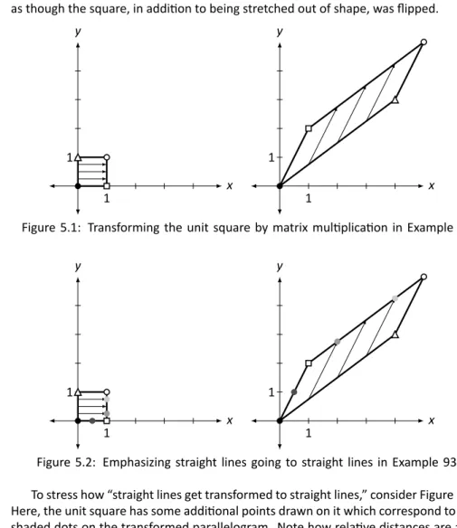
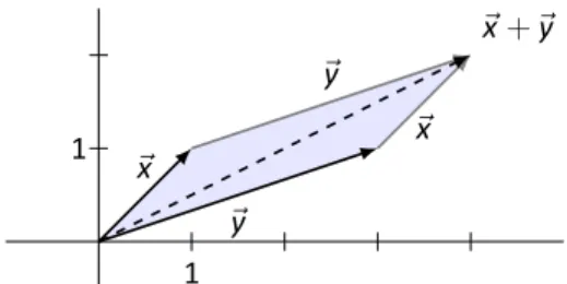
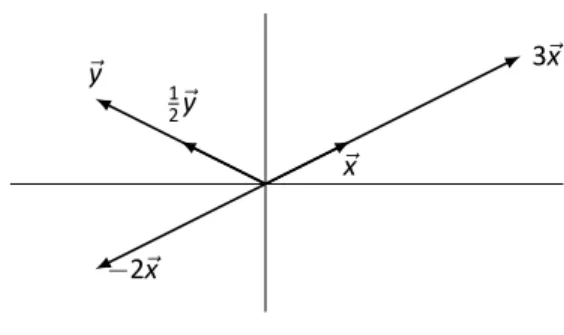
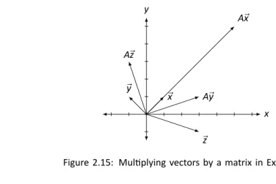
Visualizing Matrix Arithme c in 2D
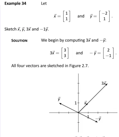
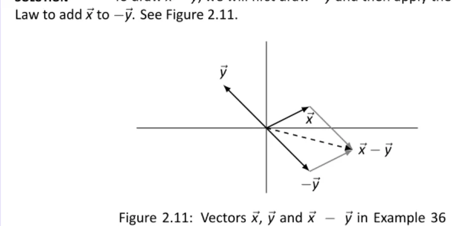
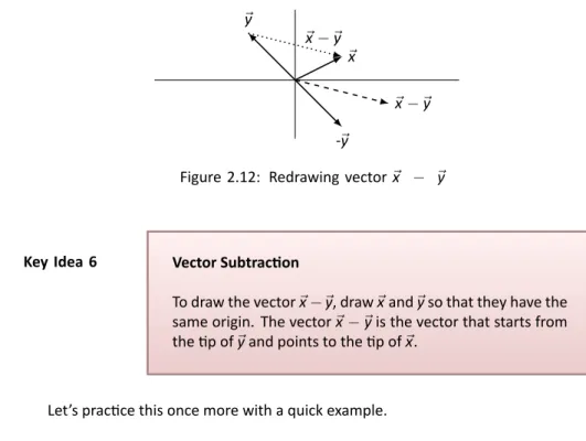
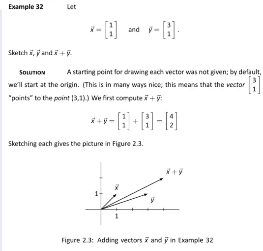
In Sec 2.1 we learned about matrix arithmetic operations: matrix addition and scalar multiplication. Finally, draw⃗x +⃗y by drawing the vector starting at the origin of e⃗yan and ending at p of⃗x. The vector⃗x−⃗is the vector that starts from p e⃗and points to p of⃗x.
Why doesn't the direction of ⃗x change more than A. We'll answer this in Section 4.1 when we learn about something called "eigenvectors". In Section 5.1, we will examine in more detail how matrix multiplication affects vectors and the entire Cartesian plane. In the next paragraph, we will take a new idea (matrix multiplication) and apply it to an old idea (solving systems of linear equations).
Vector Solu ons to Linear Systems
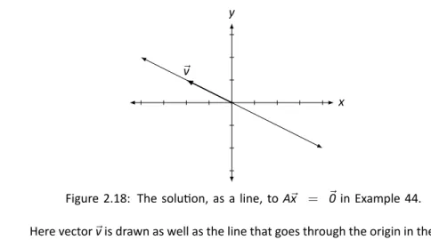
Example 44. Solve the linear system A⃗x = ⃗0for⃗x and write the solution in vector form, where. We're not done; we need to write the solution in vector form, because our solution is the vector⃗x. Therefore, a homogeneous system is always consistent; we just need to determine whether we have exactly one solution (only ⃗0) or infinitely many solutions.
Recall Key Idea 2: If the solution has any free variables, it will have infinite solutions. To write our solution in vector form, we rewrite the 1andx2in⃗xin expression ofx3andx4. To find the solution of toA⃗x =⃗0 we interpret the reduced row echelon form of the appropriate augmented matrix.
Solving Matrix Equa ons AX = B
We know how to solve it; put the appropriate matrix into reduced row form and interpret the result. You don't know that we have exactly one solution when the reduced row echelon form of A is the identity matrix. Putting this matrix into row echelon reduced form will give us X, similar to how we found⃗x.
As long as the reduced row rank form of Ai is the identity matrix, this technique works great. S To solveAX=BforX, we form the appropriate augmented matrix, put it in reduced row form, and interpret the result. Second, we have only considered cases where the reduced level form of AwasI line (and we have stated this as a requirement in our Main Idea).
The Matrix Inverse
We just saw that not all matrices are invariant.17 With this thought in mind, let's complete the set of boxes we started before the example. If not, (that is, if the first columns of the reduced row scale form are not In), then It is not inverse. 17 Hence our previous definition on; why bother calling an "inverble" if every square matrix is.
It can have infinite solutions, but it can also have no solution, and we should investigate the reduced row-echelon form of the extended matrix [A ⃗b]. In the next section we will demonstrate many different properties of inverble matrices, including several ways in which we know that a matrix is inverble. 20As strange as it may sound, it is useful to know that a matrix is reversible; Actually, the reverse is not the case.
Proper es of the Matrix Inverse
This simply states that Ais is invertible – that is, that there exists a matrix A−1 such that A−1A= AA−1 = I. We will continue to show why all the other statements basically tell us “Ais inver ble.”. It turns out that "the inverse of the transpose is the transpose of the inverse."4 We have just looked at some examples of how the transpose operation interacts with matrix arithmetic operations.5 We now give a theorem that tells us that what we saw was not accidental, but rather is always true. The part a er "is" says that we find the inverse of the matrix and then transpose it.
Now that we know some properties of the transposition opera, we are tempted to play with it and see what happens. Look at the next part of the example; what do we not know about A+AT. We can do a similar proof to show that as long as A is square, A+AT is a symmetric matrix.8 We will instead show here that if A is a square matrix, then A−AT is skew. 6 Some mathematicians use the term symmetry. 8 Why do we say it must be square.
The Matrix Trace
Now that we have defined the trace of a matrix, we need to think like mathematicians and ask some questions. The first questions that should pop into our mind should be like this: "How does the trace work with other matrix operations?" plica op, matrix inverses, and the transpose. We now formally state which equations are true when the interaction of the trace with other matrix operations is taken into account.
We close this second by wondering again why anyone would care about the trail of matrix. Our concern is not how to interpret what this "size" measurement means, but rather to demonstrate that the trace (along with the transpose) can be used to give (perhaps useful) information about a matrix.13. When looking at multiplicationATA, focus only on where the elements on the diagonal come from, since that is the only thing that determines when the trace is taken.
The Determinant
S To calculate the minorA1,3, we remove the first row and the third column ofA and then take the determinant. The minor B2,1 is found by removing the second row and first column of B and then taking the determinant. According to our definition, to calculate a minor of ann×nmatrix, we had to calculate the determinant of a (n−1)×(n−1)matrix.
Note that to calculate the determinant of an ann×n matrix, we need to calculate the determinants of an n(n−1)×(n−1) matrix. To calculate the determinant of ann×n matrix, we need to calculate the determinants of (n−1)×(n−1) matrices. a) Construct the submatrices used to compute the smaller A1,1,A1,2andA1,3. In Problems 13–24, find the determinant of the given matrix using cofactor expansion along the first row.
Proper es of the Determinant
Later we found the determinant of this matrix by calculating the cofactor expansion along the first row. If we perform an elementary row opera on a matrix, how will the determinant of the new matrix compare to the determinant of the original matrix. First, the determinant of a triangular matrix is easy to calculate: just multiply the diagonal elements.
Find the determinants of the matrices A,B,A+B, 3A,AB,AT,A−1, and compare the determinant of these matrices with their trace. Once one becomes proficient in this method, it is not that difficult to calculate the determinant of a 3×3. In Exercises 1 – 14, find the determinant of the given matrix using cofactor expansion along any row or column you choose.
Cramer’s Rule
In Section 3.4 we learned that if we consider a linear system A⃗x =⃗bwhere A is a square, if det(A)̸=0, then A is invertible and A⃗x =⃗b has exactly one solution. This is simply not done in practice; it is difficult to overcome Gaussian elimination on.24. If Cramer's rule cannot be used to find a solution, state whether or not a solution exists.
There is no definable relationship.” We might wonder if there is ever the case where a matrix - vector mul plika on is very similar to a scalar - vector mul plika on. By the same token, it has many, many applications to "the real world." A simple internet search for "applications of eigenvalues" confirms this. To do this, we form the appropriate augmented matrix and put it in a reduced row echelon form. in vector form, we have.
Proper es of Eigenvalues and Eigenvectors
This example demonstrates a wonderful fact for us: the eigenvalues of a triangular matrix are simply the entries on the diagonal. Finding the eigenvalues and eigenvectors of these matrices is not terribly difficult, but it is not "easy" either. Second, we state without justification that, given a square matrix A, we can find a square matrix such that P−1AP is an upper triangular matrix with the eigenvalues of A on the diagonal. 12Tr(P−1AP) is thus the sum of the eigenvalues; also using our Theorem 13, we know that tr(P−1AP) = tr(P−1PA) =tr(A).
Therefore, given the matrix A, we can find P such that P−1AP is an upper triangle with the eigenvalues of A on the diagonal. Finally, we found the eigenvalues of the matrices by finding the roots of the characteristic polynomial. There are several processes that can gradually transform a matrix into another matrix that is almost an upper triangular matrix (the entries below the diagonal are almost zero) where the entries on the diagonal are eigenvalues.