Fundamentals of Thermocapillary Sculpting of Liquid Nanoﬁlms and Applications to Thin Film Micro-Optics

(1)

Nanofilms and Applications to Thin Film Micro-Optics

Thesis by

Kevin Robert Fiedler

In Partial Fulfillment of the Requirements for the degree of

Doctor of Philosophy

CALIFORNIA INSTITUTE OF TECHNOLOGY Pasadena, California

2017

Defended May 5, 2017

(2)

(3)

For Sam

"It’s the song of a promising heart, of the souls that the ocean unite."

-Roy Khan

(4)

ACKNOWLEDGEMENTS

I would like to thank Dr. Troian for the opportunity to work in the Laboratory of Interstitial and Small Scale Transport (LIS²T) for six years. I have learned a great deal about fluid dynamics, heat transfer, and optics, but more importantly you have fostered a sense of independence in scientific inquiry. You let me shape and sculpt my projects while providing wisdom, support, and guidance along the way. I truly appreciate your care and concern for the present and future plans of both Sam and I.

You have also grown the group into a vibrant place with good people whom I have had the privilege to work with. To Euan McLeod, thank you for teaching me about the lab when I first arrived and how to run your experiment. To my office mates Gerry della Rocca, Zack Nicolaou, Teddy Albertson, Chengzhe Zhou, and Nick White, thank you for being my travel buddies, answering all my COMSOL questions, and your scientific insights. To my undergraduate students, Lisa Lee, Charlie Tschirhart, Tatiana Roy, Daniel Lim, Cassidy Yang, Nancy Wu, and Yanbing Zhu, thank you for your excitement while working in lab with me and letting me hone my lab safety officer speeches on you. To Dr. Thompson, thank you for installing every piece of software that I requested and keeping the computers running smoothly.

I am extremely grateful to NASA because the final four years of my graduate work were supported by a 2013 NASA Space Technology Research Fellowship (NSTRF).

The NSTRF team has been a joy to work with and has provided me an outstanding opportunity to work at the Jet Propulsion Laboratory (JPL). While at JPL, I have collaborated with the Quantum Science and Technology group which is guided by Nan Yu. It has been a privilege to work with everyone at JPL and it has been an undeniably positive aspect of my time during graduate school. In particular, I am thankful to Nan for helping shape my intuition about waveguides, resonators, and optics in general. Thank you to Thanh Le for teaching me how to couple light into waveguides and answering my practical questions in lab. Additional thanks go to the rest of the members of the Quantum Science and Technology group, especially Ivan Grudinin, Tabitha Joiner, Janice Magnuson, Vincent Huet, and Shouhua Huang.

During my time at Caltech, I have used several pieces of equipment from outside the group that were crucial for the success of my projects. In particular, I would like to thank Dr. Yunbin Guan and the Caltech Microanalysis Center for use of the Zygo NewView 600 scanning white light interferometer. I would also like to thank Dr. Rustem Ismagilov for use of his cleanroom and the Zemetrics Zegage scanning

(5)

white light interferometer. In addition, I want to thank Ali Ghaffari for use of the equipment in the Micro/Nano Fabrication Laboratory in Watson. Finally, thank you to the Molecular Materials Research Center of the Beckman Institute for the use of their profilometer, atomic force microscope, and ellipsometer.

I would also like to thank my thesis committee composed of Dr. Sandra Troian, Dr.

Kenneth Libbrecht, Dr. David Politzer, and Dr. Nan Yu. I greatly appreciate your commitment of both time and effort to be part of my committee. I am also thankful for the wisdom and guidance you have provided over the course of my graduate career. You have helped and advised me during my candidacy examination and have continued through to my final dissertation and defense.

The preparation for my graduate career started long before I set foot on Caltech’s campus and there are so many people who have helped and mentored me along my academic journey. I specifically want to thank my undergraduate advisor, Dr. Uriel Nauenberg. Uriel, thank you for opening your lab to undergraduates and teaching me about the Standard Model and the International Linear Collider. Additional thanks goes to my other undergraduate mentors, Dr. Jerry Qi, Dr. Kris Westbrook, Dr. David Rusch, Dr. Joan Gabriele, and Dr. Harvey Segur. I appreciate your efforts in teaching a young physicist about academic research. I am eternally grateful to the Boettcher Foundation for giving me the means to perform my undergraduate studies. Thank you to all my teachers from kindergarten through high school who fostered creativity and curiosity. I also want to thank Coach Boley, Coach Vande Hoef, Coach Scott, Coach Tingley, and Coach Dunn for teaching me the value of punctuality and how to tie a tie.

My time at Caltech would have been woefully incomplete without the cornucopia of friends I have encountered throughout my time in graduate school. I have been incredibly fortunate to have met Christy Jenstad who makes everything at Caltech run smoothly. I also shared the camaraderie of a lunch table who provided stories and a daily dose of vitamin D, so thank you to Fadl Saadi, John Lloyd, Erik Verlage, Ivan Papusha, Mark Harfouche, Dongwan Kim, Renee McVay, Yufeng Huang, Cris Flowers, Chengyun Hua, Sunita Darbe, and Oliver Shafaat. Outside of normal working hours I spent a large amount of time playing intramural basketball and pickup with Anandh Swaminathan, David Chen, Murat Kologlu, Sacha di Poi, Lorenzo Moncelsi, Sahin Lale, Ron Appel, and Dennis Ko. Thanks for keeping me in shape and letting me win from time to time. Thank you to my trivia buddies, Max Jones, Ioana Craiciu, Andrew McClung, Hannah Goodwin, and Sean O’Blenis, all

(6)

of whom carried the team to victory on many occasions. Thank you to all my St. Rita friends, Susan Blakeslee, Running Bear Bunch, Jo and Paul Hanson, Joe Feeney, Florian and Riza Schwandner, Jim Blackford, Jonathan Blakeslee, and Lisa Bowman, for providing stimulating discussion and excellent snacks. Thank you to all my friends from afar, Max Ederer, Steve Bloom, Chris Messick, Jess Townsend, John Chen, Kelsey and Matanya Horowitz, and Nate Mutkus. Even though I don’t see you as much as I should, you still put up with me. A special thanks goes to Chris Marotta and Lisa Mauger, who were not only excellent friends, but also provided me delicious meals while I was writing my thesis.

My family has always supported my academic endeavors and I want to express my sincere thanks to them for their continued support. Scott, thank you for keeping me honest, enlightening me about the world of finance, and perpetually finding me new book series to read. Dad, thank you for expanding my intellectual horizons, whether that was by playing "Saved by the Brain" in the car, teaching me during Math Olympiads, quizzing me on powers of two, or crushing me in backgammon.

Mom, thank you for your tireless effort and dedication. I truly could not have done it without you and you made a difference in my life in countless ways.

Last, but certainly not least, I want to thank my wife, Sam. You light up my life and give me cause to smile each time I think of you. You have been an invaluable keystone of my graduate education and I could not have done it without you. Thank you for all you do, and I look forward to our future adventures both in life and science. I love you more than words can express and so this thesis is dedicated to you.

(7)

ABSTRACT

This doctoral thesis describes experimental work conducted as part of ongoing efforts to identify and understand the source of linear instability in ultrathin liquid films subject to large variations in surface temperature along the air/liquid interface.

Previous theoretical efforts by various groups have identified three possible physical mechanisms for instability, including an induced surface charge model, an acoustic phonon model, and a thermocapillary model. The observed instability manifests as the spontaneous formation of arrays of nano/microscale liquid protrusions arising from an initially flat nanofilm, whose organization is characterized by a distinct in-plane wavelength and associated out-of-plane growth rate. Although long range order is somewhat difficult to achieve due to thin film defects incurred during preparation, the instability tends toward hexagonal symmetry within periodic domains achieved for a geometry in which the nanofilm is held in close proximity to a cooled, proximate, parallel, and featureless substrate.

In this work, data obtained from a previous experimental setup is analyzed and it is shown how key improvements in image processing and analysis, coupled with more accurate finite element simulations of thermal profiles, lead to more accurate identification of the fastest growing unstable mode at early times. This fastest growing mode is governed by linear instability and exponential growth. This work was followed by re-examination of real time interference fringes using differential colorimetry to quantify the actual rate of growth of the fastest growing peaks within the protrusion arrays. These initial studies and lingering questions led to the introduction of a new and improved experimental setup, which was redesigned to yield larger and more reproducible data sets. Corresponding improvements to the image analysis process allowed for the measurement of both the wavelength and growth rate of the fastest growing mode simultaneously. These combined efforts establish that the dominant source of instability is attributable to large thermocapillary stresses.

For the geometry in which the nanofilm surface is held in close proximity to a cooled and parallel substrate, the instability leads to a runaway process, characterized by exponential growth, in which the film is attracted to the cooled target until contact is achieved.

The second part of this thesis describes fabrication and characterization of microlens arrays and linear waveguide structures using a similar experimental setup. However, instead of relying on the native instability observed, formation and growth of liquid

(8)

shapes and protrusions is triggered by pre-patterning the cooled substrate with a desired mask for replication. These preformed cooled patterns, held in close proximity to an initially flat liquid nanofilm, induce a strong non-linear response via consequent patterned thermocapillary stresses imposed along the air/liquid interface.

Once the desired film shapes are achieved, the transverse thermal gradient is removed and the micro-optical components are affixed in place naturally by the resultant rapid solidification. The use of polymer nanofilms with low glass transition temperatures, such as polystyrene, facilitated rapid solidification, while providing good optical response. Surface characterization of the resulting micro-optical components was accomplished by scanning white light interferometry, which evidences formation of ultrasmooth surfaces ideal for optical applications. Finally, linear waveguides were created by this thermocapillary sculpting technique and their optical performance characterized. In conclusion, these measurements highlight the true source of instability in this geometry, and the fabrication demonstrations pave the way for harnessing this knowledge for the design and creation of novel micro-optical devices.

(9)

PUBLISHED CONTENT AND CONTRIBUTIONS

1K. R. Fiedler, and S. M. Troian, “Early time instability in nanofilms exposed to a large transverse thermal gradient: improved image and thermal analysis”, J. Appl.

Phys.120, 205303 (2016),

KRF assisted with the design of the project, remeasured characteristic instability wavelengths, improved the numerical simulations, prepared draft plots and figures, and participated in the writing of the manuscript.

2K. R. Fiedler, E. McLeod, and S. M. Troian, “Differential colorimetry measurements of instability growth in nanonfilms exposed to a large transverse thermal gradient”, To be submitted to J. Appl. Phys. (May 2017),

KRF recomputed the interference fringe spectra of nanofilms to establish local film thickness, measured the peak heights as a function of time and associated growth rates, compared results to theoretical predictions of the thermocapillary model, prepared draft plots and figures, and participated in the writing of the manuscript.

3K. R. Fiedler, and S. M. Troian, “Optical observations of a long-wavelength thin film instability driven by thermocapillary forces”, To be submitted to Phys. Rev.

E. (2017),

KRF assisted with the design of the project, built the experimental setup, measured the wavelength of the fastest growing mode, performed the numerical simulations, prepared draft plots and figures, and participated in the writing of the manuscript.

4S. W. D. Lim, K. R. Fiedler, C. Zhou, and S. M. Troian, “Converging and diverg- ing microlens arrays by spatiotemporal control of thermocapillary forces”, To be submitted to Appl. Phys. Lett. (2017),

KRF assisted with the design of the project, measurements obtained, discussions of the results, and preparation of the manuscript.

5K. R. Fiedler, S. W. D. Lim, Y. Zhu, and S. M. Troian, “Fabrication of microdevices through thermocapillary sculpting of molten polymer nanofilms”, In preparation (2017),

KRF assisted with the design of the project, built the fabrication setup, assisted with device characterization, prepared draft plots and figures, and participated in the writing

(10)

of the manuscript.

6K. R. Fiedler, Y. Zhu, T. Le, N. Yu, and S. M. Troian, “Characterization of linear optical waveguides formed by thermocapillary sculpting of nanoscale polymer melt films”, In preparation (2017),

KRF assisted with the design of the project, fabricated and characterized the waveguides, performed the numerical simulations of waveguide properties, prepared draft plots and figures, and participated in the writing of the manuscript.

(11)

LIST OF ILLUSTRATIONS

Number Page

1.1 Basic nanofilm instability geometry . . . 1

1.2 Basic nanofilm deformation geometry with a patterned top plate . . . 6

2.1 Schematic of the instability geometry . . . 9

2.2 Instability geometry in SC model . . . 19

2.3 Instability geometry in AP model . . . 25

2.4 Instability geometry in TC model . . . 30

3.1 Diagram of the experimental setup . . . 39

3.2 Illustration of the image analysis process . . . 44

3.3 Illustration of the image analysis process showing temporal dependence of the measured wavevector . . . 45

3.4 Impact of defects during image analysis and wavelength measurement 46 3.5 Comparison of the current wavelength measurements to the wavelengths measured by McLeodet al. . . . 48

3.6 Computational geometry and boundary conditions for the finite element simulations of the temperature within the experimental setup . . 49

3.7 Finite element simulation of the temperature in the experimental setup 52 3.8 Comparison of the temperature drops computed with the current thermal simulations to the temperature drops computed by McLeod et al. . . . 55

3.9 Comparison of the analyzed experimental data with improved image and thermal analysis to the AP and TC model predictions . . . 57

4.1 Diagram of the experimental setup used for optical observation . . . 62

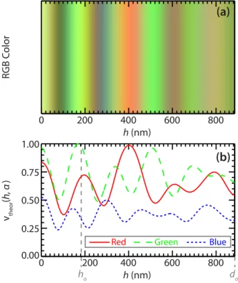
4.2 Theoretical interference fringe color for films with different thicknesses 68 4.3 Images of peak growth as a function of time . . . 71

4.4 Analysis of peak growth as a function of time and example of growth rate measurement . . . 72

4.5 Nondimensional growth rate plotted as a function of nondimensional wavelength . . . 73

4.6 Nondimensional growth rates plotted as functions of normalized gap ratio . . . 74

5.1 Diagram of the redesigned experimental setup . . . 83

(15)

5.2 Diagram of the computational domain for the temperature simulations

of the redesigned experimental setup . . . 90

5.3 Effect of a sinusoidal deformation to the molten nanofilm on the temperature simulations of the experimental setup . . . 93

5.4 Plots of the derived peak fitting function and comparison to Gaussian and Lorentzian peaks . . . 98

5.5 Illustration of the image analysis process using the derived fitting function . . . 103

5.6 Normalized wavevector plotted as a function of time for every experimental run . . . 104

5.7 Diagram of the instability geometry . . . 105

5.8 Wavelengths normalized by the SC model . . . 111

5.9 Wavelengths normalized by the AP model . . . 112

5.10 Wavelengths normalized by the TC model . . . 113

5.11 Nondimensional growth rate plotted as a function of the nondimensional wavelength . . . 114

5.12 Growth rates normalized by the SC model . . . 115

5.13 Growth rates normalized by the AP model . . . 116

5.14 Growth rates normalized by the TC model . . . 117

6.1 Basic MicroAngelo experimental setup for microlens array fabrication 125 6.2 Optical images of MLAs produced on silicon wafers . . . 126

6.3 Diagram of the full MicroAngelo experimental setup . . . 129

6.4 Topographies of fabricated microlens arrays . . . 130

6.5 Geometry of the mask used in MLA finite element simulations . . . . 137

6.6 Comparison of experimental MLA cross sections to numerical simulation cross sections . . . 139

6.7 Diagram of the Shack-Hartmann wavefront sensor setup . . . 140

6.8 Caldera-like MLA transmitted light profiles and SHWS image . . . . 142

7.1 Schematic of the experimental setup used to fabricate waveguides . . 145

7.2 Images of a fabricated waveguide . . . 147

7.3 Profilometer scans of waveguide cross sections . . . 148

7.4 Diagram of optical characterization setup . . . 149

7.5 Optical images of the TE modes from waveguide #2 . . . 151

7.6 Optical images of the TM modes from waveguide #3 . . . 151

7.7 Computational domain and simulated waveguide modes . . . 154

7.8 Comparison between MicroAngelo and rectangular waveguides . . . 156

(16)

7.9 Single mode MicroAngelo waveguide geometries . . . 158

7.10 Polarization window of waveguide #2 . . . 159

A.1 SU-8 photomask example . . . 179

A.2 Wafer cleaving diagram . . . 183

B.1 Instability geometry in EHD model . . . 191

(17)

LIST OF TABLES

Number Page

2.1 Dimensional wavelengths and growth rates for each proposed model . 32 3.1 Material constants for the SC model . . . 35 3.2 Material constants for the AP model . . . 36 3.3 Material constants for the TC model . . . 37 3.4 Fit parameters of Eq. (3.1) for the curves shown in Fig. 3.2(d) . . . . 42 3.5 Fit parameters of Eq. (3.1) for the curves shown in Fig. 3.3(d) . . . . 42 3.6 Listing of domain sizes and thermal conductivities for the simulation

domain shown in Fig. 3.1 and Fig. 3.6 . . . 50 3.7 Listing of all analyzed experiments with their parameters and analysis

results . . . 60 4.1 Experimental parameter ranges for the experiments where the growth

rate was measured . . . 64 4.2 Cauchy coefficients for the materials in the experimental setup . . . . 66 4.3 Growth rate analysis parameters and derived values . . . 76 4.4 Measured growth rates for each experimental run reported in units of

10⁻⁴1/s . . . 77 5.1 Sizes and thermal conductivities for each domain in the numerical

simulations of temperature within the experimental setup . . . 91 5.2 Fitting constants for the curves shown in Fig. 5.5(c) . . . 102 5.3 Parameters for the experimental runs and material properties for 1.1k

MW polystyrene . . . 108 5.4 Scaled wavelengths,Λ, and growth rates,β, for each of the proposed

models . . . 109 5.5 Parameters and thermal conductivities for the thermal simulations . . 121 5.6 Image analysis parameters and measured wavelengths and growth rates122 5.7 Material properties at the temperature of each experimental run . . . 123 6.1 Parameter values for the fabricated microlens arrays . . . 131 6.2 Measured and derived values of the fabricated microlens arrays . . . 135 6.3 List of parameters for the simulation of microlens evolution . . . 138 7.1 Experimental parameters for each of the four fabricated waveguides . 146 7.2 Fitting constants for the measured waveguide cross sections for each

of the waveguides . . . 149

(18)

7.3 Coupling efficiency lower bounds and TM extinction ratio measurements . . . 152 A.1 Abbe refractometer calibration data and PS refractive index . . . 186

(19)

NOMENCLATURE

This is a compilation of the abbreviations and symbols which are used in this work. Generally, dimensional variables are lower case letters while dimensionless variables are the corresponding upper case letters. In the case of operators, the nomdimensional analogs typically have a tilde over them. Within the body of this document, certain variables will be subscripted byi. This subscript will typically represent different layers in the system, primarily either "film" or "air".

[·] Denotes a difference across the air/nanofilm interface α RGB channel index

α4 First aspheric coefficient β Nondimensional growth rate

∆T^curr Temperature drops computed using the expanded domain in Ch. 3

∆T^orig Temperature drops computed in Ref. [1]

δφ Perturbed electric potential

∆T_out Difference between the heater and chiller setpoints

∆T_sin Temperature drop across the sinusoidally perturbed bilayer δD® Perturbed electric displacement field

δE® Perturbed electric field

δhk⁰ Fourier coefficients describing the current interface height

∆l Fabry-Pérot etalon change in length

∆t Time step between peak observation images δ Normalized mask pin height

∆T Temperature difference between the bounding plates δj(λ_opt) Optical phase

QÛ_ITO Volumetric heat flux density within the ITO heater Long wavelength expansion parameter

Γ Dimensionless surface tension

γ Surface tension of the fluid/air interface Γc Characteristic scale of the surface tension γT Thermocapillary coefficient

ˆ

n Unit normal vector at the nanofilm/air interface tˆ Tangential unit vector

~ Reduced Planck’s constant κ Thermal conductivity ratio

(20)

λ_opt Wavelength of optical illumination λo Lateral spacing of instability protrusions

E Rate of strain tensor

Mj,j+1 Optical transmission matrix from layer j to layer j+1 Mj Optical transmission matrix through layer j

T Stress tensor

T^em Maxwell stress tensor F (k,t) Peak fitting function

G (k) Gaussian fitting function L (k) Lorentzian fitting function

T Temperature

T₊ Temperature measured by the thermocouple on the chiller T− Temperature measured by the thermocouple underneath the heater T_C Temperature of the cooled top plate

T_H Temperature of the heated bottom plate

T_Int Temperature at the interface of the molten nanofilm T_g Glass transition temperature

µ Dynamic viscosity of the fluid

∇_s Surface gradient

∇_k Horizontal components of the gradient

ν Mode order

ω Frequency of an oscillator Ca Modified capillary number M a Modified Marangoni number

Q Acoustic quality factor φ Electric potential

φ^o Base state electric potential

Φ_c Characteristic scale of the electric potential

Φ⁰_c Alternative electric potential scale in the EHD model Φ_o Applied potential difference

Π MicroAngelo mask pitch ρ Density of the fluid

σ Surface charge density at the fluid/air interface σ_free Free charge density at an interface

τ Dimensionless time

v_exp(x,y,t, α) Experimental fringe color values

(21)

v_theor(h, α) Fringe color values

Θ Nondimensional temperature

θ Angle between principal axes and the raw data axes

˜v_theor(h, α) Normalized fringe color values ε Relative permittivity

εo Permittivity of free space D® Electric displacement field E® Electric field

E®^o Base state electric field

f®_body Body forces acting on the bulk of the fluid K® Nondimensional wavevector of the instability

®k Wavevector of the instability q® Heat flux density

u® = (u,v,w) Velocity field within the nanofilm u®k = (u,v) Horizontal components of the velocity

fδh Nondimensional perturbation used in linear stability analysis f∇_s Dimensionless surface gradient

∇f_k Dimensionless lateral gradient φei Nondimensional electric potential e®

Ei Nondimensional electric field A Amplitude of peak fitting function a Width of an infinite square well Alens Individual MLA lens area

A_wg Waveguide amplitude

bo Growth rate of peak fitting function

C^AP Fitting constant for the material constants in the AP model C^TC Fitting constant for the material constants in the TC model

cp Specific heat capacity

D Dimensionless gap separation

d1 MicroAngelo mask pin or block height d2 MicroAngelo mask depression height Dlens Characteristic MLA lens diameter

do Separation between bounding plates

Dp MicroAngelo mask pin or depression diameter D_wg Gaussian decay of waveguide envelope

Eν Energy of modeν

(22)

f₁ Larger microlens focal length f2 Smaller microlens focal length

Farray Fresnel number of the microlens array Flens Fresnel number of an individual microlens

fp Mask pin protrusion function

G Functional form of the mask topography g(x,y,t,h) Peak height cost function

H Dimensionless film thickness

h(x,y,t) Interface position between molten nanofilm and air h_meas(x,y,t) Measured peak height as a function of time

h_paste Thermal paste thickness

hpk(t) Peak height during film growth ho Initial film thickness

I Measured intensity signal

I(λ_opt) Intensity spectrum of the halogen light source IR Reflected intensity from a Fabry-Pérot etalon

k Thermal conductivity

k₊ Right half maximum point of peak fitting function k− Left half maximum point of peak fitting function k_max Upper bound for the peak fitting function

kmin Lower bound for the peak fitting function ko Maximum point of peak fitting function

l Fabry-Pérot etalon length

m Mass of a particle in an infinite square well n Index of refraction

P Dimensionless pressure p Pressure within the fluid

P_ac Nondimensional acoustic pressure used in the AP model p_ac Acoustic pressure used in the AP model

Pel Nondimensional electric pressure used in the SC model pel Electric pressure used in the SC model

Pc Characteristic scale of the pressure in the fluid Pr Prandtl number

R(λ_opt,h) Reflectance from a multilayer stack

R₁ Microlens radii of curvature along the larger principal axis R₂ Microlens radii of curvature along the smaller principal axis

(23)

r_paste Thermal paste radius

rj,j+1 Fresnel amplitude reflection coefficient

Re Reynolds number

rn(x,y) Random number generator in COMSOL S

®k,t

Power spectral density

S_α(λ_opt) Spectral responsivity of the camera

t_final Last time which was analyzed in the wavelength analysis t_meas Time of initial wavelength measurement

tf Final time of the peak observation

t_ref Time stamp of the image which was used as the reference image tj,j+1 Fresnel amplitude transmission coefficient

U,V,W Dimensionless fluid velocities

uc Characteristic lateral scale of the flow velocity up Speed of sound in the molten nanofilm

W(k) Background plus peak fitting function

wc Characteristic vertical scale of the flow velocity w_wg Waveguide width

x⁰,y⁰ Microlens principal axes

X,Y,Z Dimensionless position variables x_pk,y_pk Peak location as a function of time

xf,yf Location of peak at final time

xo,y_o Coordinates of the microlens vertex in raw data coordinates zj Thickness of layer j

zmax Height of individual microlens

AP Abbreviation for the acoustic phonon model AR Asphericity ratio

EHD Abbreviation for the electrohydrodynamic model

HeNe Helium neon

IPA Isopropyl alcohol ITO Indium tin oxide

JPL Jet Propulsion Laboratory

LIS²T Laboratory of Interstitial and Small Scale Transport NSTRF NASA Space Technology Research Fellowship

PBS Polarizing beam splitter PDMS Polydimethylsiloxane

PID Proportional integral derivative

(24)

PMMA Poly(methyl methacrylate)

PS Polystyrene

RGB Red green blue RMS Root mean square

RTD Resistance temperature detector

SC Abbreviation for the surface charge model SHWS Shack-Hartmann wavefront sensor

SSR Sum of squared residuals

TC Abbreviation for the thermocapillary model

TE Transverse electric electromagnetic wave polarization TM Transverse magnetic electromagnetic wave polarization

(25)

C h a p t e r 1

INTRODUCTION

Almost twenty years ago, the spontaneous formation of pillars from a molten nanofilm in a confined geometry subject to a transverse thermal gradient was observed by Chou and Zhuang [2, 3]. In their experiment, solid polymeric nanofilms were spun coat on a silicon wafer with an initial film thickness,ho, of approximately one hundred nanometers. Subsequently, another silicon wafer was overlaid on this coated wafer. To ensure an air gap between the top surface of the nanofilm and the overlaid wafer, the wafer was patterned with spacers which determined the total plate separation distance,do, and this distance was typically on the order of several hundred nanometers to a micron. A schematic of their experimental setup is shown in Fig. 1.1. Upon heating, the temperature of the system was raised significantly above the glass transition temperature so that the film was in a molten state. After deformation times ranging from 5 to 80 minutes, the molten film was allowed to solidify and hexagonal arrays of pillars with lateral spacing on the order of microns were observed after the bounding plate was removed. These pillars had spanned the air gap during deformation and contacted the top plate, creating pillars with flat tops and fairly vertical sidewalls. At the time, there was no explanation for this phenomenon. It has since generated controversy over the dominant physical mechanism that causes the molten nanofilm to be unstable in this system. Several possibilities have been put forth and will be discussed in turn.

Figure 1.1: Basic nanofilm instability geometry

λo Air

Molten Nanofilm Heater ho

do ∆T

Schematic of the nanofilm geometry. The molten nanofilm is bounded from below by a heated substrate and from above by an air layer. The air layer is bounded from above by a plate where the total plate separation,d_o, is typically on the order of a micron, while the initial film thickness,h_o, is on the order of hundreds of nanometers. The temperature drop from bottom to top plates is typically on the order of 10 °C. The lateral spacing of the protrusions,λ_o, is on the order of microns to tens of microns.

(26)

1.1 Previous Instability Investigations: Surface Charge (SC) Model

The first model proposed to explain the instability of this film was put forward by Chou and Zhuang [2, 3]. Their model treats the molten nanofilm from the perspective of fluid dynamics wherein it is linearly unstable to perturbations. They hypothesized that charges at the nanofilm’s free interface induce image charges in the heating and cooling plates. The combined effect of these charges creates an electric field which exerts a destabilizing electrostatic stress on the interface to overcome the stabilizing force of surface tension. Due to its dependence on interfacial charge density, this model will be referred to as the surface charge (SC) model. Interestingly, they noted that in addition to electrical effects, thermal effects might be playing a role because if the molten nanofilm was not bounded from above by the overlaid wafer, then the pillars were not observed after solidification of the film. However, they did not intentionally impose a thermal gradient across the system with active cooling of the top plate. Additionally, they estimated that the critical numbers for cellular convection driven by thermal effects such as Rayleigh-Bénard and Bénard- Marangoni convection were far too small for instability to occur. Regardless, the spatial period of the observed hexagonal arrays showed an unexplained dependence on the temperature of the system.

1.2 Previous Instability Investigations: Acoustic Phonon (AP) Model

Nearly simultaneously with the work of Chou and Zhuang, Schäffer and co-workers investigated an instability in a similar geometry [4–6]. As before, they spun coat polymeric nanofilms onto silicon substrates and placed them in a confined geometry through the use of spacers. The key difference from the experiments of Chou and Zhuang is that in the experiments of Schäfferet al. the top plate was actively cooled.

The cooler top plate was held at a temperature above the glass transition temperature of the polymer and the temperature difference between the bounding plates was on the order of 10 °C. The setup was subjected to this externally imposed transverse thermal gradient overnight and then the nanofilm was solidified. Once again, hexagonal arrays of pillars with flat tops were observed upon removal of the top plate.

To rule out any electrostatic effects, both of the bounding plates were electrically grounded. As Chou and Zhuang did, Schäfferet al. calculated the Rayleigh-Bénard and Bénard-Marangoni numbers in nanofilm experiments and found that they were many orders of magnitude smaller than the critical ones required for instability. To explain the observed results, they suggested that the instability might be due to an acoustic phonon mechanism leading to periodic modulation of the acoustic pressure

(27)

within the film. In this model, acoustic phonon reflections create a net acoustic pressure which destabilizes the interface and causes protrusions to grow. Specifically, they conjectured that phonons with low frequency would be coherently reflected off the nanofilm/air interface while high frequency phonons would be unaffected by the interface and conduct most of the heat flux through the system. These low frequency phonon reflections would then contribute a significant destabilizing radiation pressure which overpowers surface tension to create protrusions. This model will be referred to as the acoustic phonon (AP) model.

Following a derivation of a complete hydrodynamic theory describing the instability in terms of the radiation pressure, they used linear stability analysis to derive a result for the characteristic spacing of the film’s fastest growing mode,λo, as a function of the initial film thickness, ho, total plate separation, do, and temperature drop,

∆T. They then performed a set of experiments to probe the functional dependence of λo on do by introducing a tilt between the bottom and top plates to measure a range of do for a single run at a givenho value. They repeated this procedure for several values ofho. By fitting one of the parameters in their theory, they were able to find agreement between the experimental data and the theoretical prediction for λo over a limited range of do. Due to their decision to vary do through substrate tilt, they were only able to measure values of do that varied by a factor of three in a given experimental run and only achieved a range of a factor of six over all the experimental runs. Furthermore, the induced substrate tilt induced an extra lateral gradient which was not included in their model. More problematic for their comparisons to the wavelength predicted by linear stability theory, the values that they reported for λo were all measured far outside of the linear regime because the deformations were allowed to contact the top plate and solidify. Prolonged contact with the top plate can drastically changed the pattern morphology through coarsening or van der Waals interactions which were not considered in the AP model. Furthermore, several measurements were made in regions where growth of structures was nucleated by defects which would also invalidate the comparison of the experimental data to linear stability theory.

Following in this vein, Penget al. demonstrated formation of hexagonal arrays from heated polymeric nanofilms in confined geometries [7], similar to what had been previously reported by Schäffer et al.. They then took the hexagonal patterns and transferred them to a stamp made of polydimethylsiloxane (PDMS) which could then be used for future microfabrication steps. Even though there was strong ordering in

(28)

these systems, Penget al. did not measure the spacing of their arrays as a function ofho,do, or∆T, nor did they compare to any proposed model.

1.3 Previous Instability Investigations: Thermocapillary (TC) Model

Several years later, Dietzel and Troian began to investigate these issues and re- evaluated the assumptions of the SC and AP models [8–10]. In particular, they noted that phonon mean free paths on the order of ten to one hundred nanometers required for coherent reflection from the film interface in the AP model have only been measured in solid polymer systems at temperatures far below the glass transition temperature. They conclude that it is unlikely that molten amorphous films would be able to support the long attenuation lengths due to the increased mobility of the polymeric system above the glass transition temperature. They also reexamined the assertion by both Chou et al. [2] and Schäffer et al. [6] that the critical numbers which typically govern Bénard-Marangoni convection would be too small in nanofilm experiments for instability. Their theoretical and computational work [8–10] has indicated that the instability represents a new limit of the long wavelength Bénard-Marangoni instability, distinguished by extremely large thermocapillary forces and negligible hydrostatic forces, which is not governed by the traditional critical numbers. The underlying concept for this model is that protrusions will be slightly cooler than valleys and they will have a correspondingly higher surface tension. This gradient in surface tension between peaks and valleys creates a destabilizing shear stress along the interface which causes lateral flow and, through incompressibility, out of plane protrusion growth. This model will be referred to as the thermocapillary (TC) model. Based on the TC model, they also derived a prediction for the characteristic spacing of the film’s fastest growing mode, λo, as a function of the initial film thickness, ho, total plate separation, do, and temperature drop,∆T, and compared it to the experimental data of Schäfferet al. [4–6] and concluded that the TC model was consistent with the experimental data to that point, and could potentially play a critical, if not dominant, role in the film evolution.

Shortly thereafter, McLeod et al. performed a series of experimental wavelength measurements to further investigate the underlying instability mechanism [1]. These experiments focused on improving the experimental measurement techniques to more accurately compare the measured wavelengths to the predictions of linear stability theory from the SC, AP, and TC models. In particular, they performed in situ optical measurements of the instability during the deformation process to

(29)

measureλowhen the deformations were small compared to the initial film thickness and well before the protrusions contacted the top plate. Furthermore, none of the previous experiments had measured or calculated the temperature drop across the nanofilm/air bilayer. Due to the minute size of the gap, it is impossible to directly measure the temperature in the gap using a thermocouple. Instead, the difference between heater and chiller setpoints was taken to be equal to the temperature drop across the bilayer. McLeodet al. improved upon this procedure by performing finite element simulations of the experimental setup based on thermocouple measurements to compute the temperature difference across the bilayer. They also performed many more experimental runs than Schäffer et al. [4–6] and swept a much larger range of do, ho, and ∆T. With this experimental setup, they found that the experimental data for the measured wavelength was most consistent with the TC model, but that close numerical agreement required the thermal conductivity of the polymer nanofilm to be fit. The required value for the vertical, out-of-plane polymer thermal conductivity was found to be five times larger than the bulk value. It was originally postulated that polymer chain alignment could account for the increase in thermal conductivity, but this hypothesis is problematic for two reasons. First, in cases where polymer alignment has been observed [11], the polymer used was well above the entanglement molecular weight where long chains can interact. Conversely, the polymer used in the work of McLeodet al. was well below the entanglement limit so a potential alignment mechanism is not clear. Second, the increase in thermal conductivity of spin coated polymeric thin films has been observed in the lateral direction, not the vertical one [12]. As such, even with the improved experimental setup, there remained discrepancies between the experimental measurements and the theoretical predictions.

1.4 Pattern Replication through Controlled Film Deformation

Concurrently with the fundamental science investigations into the underlying instability mechanism presented above, there has been research into controlling and localizing feature deformation as a potential manufacturing technique. To do this, the locally flat top plate from Fig. 1.1 was patterned with another set of features which stretch toward the nanofilm in addition to the spacers. A schematic of this geometry is shown in Fig. 1.2. In all three models, the presence of a patterned mask on the top plate will localize deformation and allow for control of the film because the mask changes the local gap width.

The first demonstration of pattern replication in these types of geometries was by

(30)

Figure 1.2: Basic nanofilm deformation geometry with a patterned top plate

Air Molten Nanofilm

Heater ho

do ∆T

Schematic of the nanofilm geometry where the feature deformation is localized by patterns on the top plate. The ranges for the experimental parameters are the same as for Fig. 1.1.

Chou and co-workers where they patterned the top plate with a triangle, a square and the text "PRINCETON" [2, 13]. In each case, they observed pillar arrays in the shape of the patterned mask and virtually no deformation in the regions outside the mask. In a related study, Chouet al. observed that the film would completely cover the applied mask if it was closer in proximity to the initial film height [14].

In this case, the pillar arrays merged into a continuous feature which replicated the mask. Similarly, Schäfferet al. demonstrated pattern replication of hexagonal arrays, square arrays, and lines with feature sizes as small as 500 nm [4, 15]. In all of the cases just discussed, the features were allowed to grow until they contacted the mask. This meant that all the features had flat tops due to their interaction with the mask. Instead of allowing the film to grow unchecked, McLeod and Troian stopped the film deformation before it interacted with the mask to produce a square array of curved lenses [16]. This experimental work corresponds more closely with the schematic in Fig. 1.2 than the previous studies which would have touched the mask protrusions. The ability to localize nanofilm deformations using patterned masks opens up a new avenue for the fabrication of unique structures with ultrasmooth surfaces. This system profiles as a novel lithographic technique, but more work needs to be done to understand the advantages and limitations.

1.5 Thesis Outline

In the spirit of the previous studies mentioned above, this thesis seeks to investigate and understand the residual discrepancies between the experimental instability data and the theoretical predictions. It also seeks to deform nanofilms into structures through the use of patterned masks on the top plate and then characterize their properties. As such, the remainder of this thesis is organized as follows. In Ch. 2, the equations describing the distinct sources of instability proposed to explain the spontaneous nanofilm deformation are reviewed. For each of the three previously proposed linear instability models (SC, AP, and TC), predictions for the fastest

(31)

growing mode and its corresponding wavelength and growth rate are compared. The next three chapters focus on the experimental and numerical work which investigated the dominant physical mechanism driving this thin film instability. Specifically, in Ch. 3 improved analysis techniques for image analysis and thermal simulation are detailed to improve the comparison of measured wavelengths to the AP and TC models. In Ch. 4 the growth of protrusions are measured as a function of time using colorimetric information derived from thin film interference fringes. The resulting growth rates are compared to the predictions of the TC model. Next, an improved experimental setup is detailed and the instability measurements which were made with it are described in Ch. 5. The results of these experiments strongly indicate that the dominant instability mechanism is caused by interfacial thermocapillary stresses.

After this, the next two chapters focus on the fabrication of two kinds of micro-optical components using thermocapillary forces. First, microlens arrays were fabricated and characterized. The results of this study are presented in Ch. 6. Beyond microlens arrays, linear optical waveguides were also fabricated and characterized and this work is described in Ch. 7. Finally, Ch. 8 describes conclusions from the thesis and suggests experimental improvements for future studies.

(32)

C h a p t e r 2

REVIEW AND COMPARISON OF THREE THIN FILM INSTABILITY MODELS

As mentioned above in Ch. 1, nanofilms on a heated substrate are found experimen- tally to be unstable. To better understand this phenomenon, several groups have approached this process theoretically by modeling it as a fluid instability. All of the proposed mechanisms for this phenomenon revolve around thin film hydrodynamic instability theory. They differ in the specific driving force which destabilizes the film against the force of surface tension but possess several unifying features. In this chapter we review the three proposed mechanisms and synthesize the previous work into one derivation which has consistent notation and serves to highlight the origin and influence of the various driving forces. We also present the derived expressions which the later experimental results are compared with in Ch. 3, Ch. 4, and Ch. 5.

The remainder of this chapter is organized as follows. In Sec. 2.1, a thin film height evolution equation is derived for the position of the nanofilm/air interface,h(x,y,t), starting from the basic equations of fluid mechanics. Subsequently in Sec. 2.2 these equations are nondimensionalized and simplified using the long wavelength approximation. Then in Sec. 2.3 linear stability analysis is applied for each of the three proposed models. The results of the linear stability analysis give tangible predictions for the wavelength and growth rate of the fastest growing mode.

2.1 Fluid Dynamics Governing Equations

To specify the system completely, we define the domain, the governing equations, and the boundary conditions for the system. As mentioned in Ch. 1, the system of interest is a free surface molten nanofilm bounded by an air layer. Note that this derivation is only concerned with the fluid dynamics of the liquid nanofilm and not the air layer. Due to the large difference between the density and viscosity of the liquid nanofilm and the density and viscosity of the air layer only the dynamics of the fluid layer are explicitly considered.

2.1.1 Nanofilm Instability Geometry

The domain which we will consider is a thin liquid film which has an initial height ho. This can also be interchangeably referred to as the film thickness. The film is

(33)

Figure 2.1: Schematic of the instability geometry

λ_o Air

z x

y h Molten Nanofilm

o

h(x, t) do

×

The molten nanofilm is bounded from below by a heated substrate and from above by a plate which is cooled. The total plate separation is denoted byd_o, while the initial film thickness is denoted by h_o. The temperature drop from hot to cold plates is denoted by∆T=TH−TCand the lateral spacing of the protrusions is denoted byλ_o.

supported from below by a rigid, impermeable, heated substrate. The upper surface of the film is a free interface and a distance do from the bottom of the film there exists a cooled, upper plate which constrains the system in the vertical direction.

2.1.2 Mass and Momentum Continuity Equations

There are two differential equations which we will use to describe this system.

The first differential equation is the mass continuity equation. We will assume incompressible flow and the resulting equation is

∇ · ®u= 0. (2.1)

In this equationu®= (u,v,w)is the velocity of the molten nanofilm as a function of space and time. The other differential equation which governs the fluid dynamics in the molten layer is the Navier-Stokes equation where we have assumed that the fluid is Newtonian. This equation physically represents the conservation of momentum and has the form

ρDu®

Dt =−∇p+ µ∇²u®+ f®body, (2.2) where ρ is the density of the fluid, p is the pressure, µis the shear viscosity and f®_body is the effect of body forces on the fluid. The most common body force which acts on fluids is gravity. Previous theoretical work [8–10] has estimated that gravity is negligible in nanofilm experiments due to the minuscule height scales. As such, fbody will be set to zero for the remainder of this work. The notation for the time derivative on the left hand side of the equation is the convective, or material, derivative and is defined by

D Dt ≡ ∂

∂t +u®·∇. (2.3)

(34)

This describes how a quantity changes in time as well as local changes due to variations along the local velocity field.

2.1.3 Fluid Velocity and Pressure Boundary Conditions

With the governing equations specified, we now outline the boundary conditions required for solution ofu®andp. At the bottom of the liquid layer (z =0 in Fig. 2.1) there is a no-slip and impenetrability condition with the solid wall

u®(z =0)=0. (2.4)

At the free interface there is both a kinematic boundary condition and an interfacial stress balance. The kinematic boundary condition relates the vertical component of the fluid velocity to the change of the film height at the interface

w(z= h)= ∂h

∂t +u®k ·∇_kh. (2.5)

The subscriptkdenotes that only the ˆxand ˆycomponents of the subscripted quantity should be included in the expressions. Consequently, the horizontal velocity is defined by

u®k ≡ uxˆ+vy.ˆ (2.6)

Similarly, the horizontal gradient,∇_k, is composed of the derivatives solely in the ˆx and ˆydirections. In other words,

∇_k = xˆ ∂

∂x +yˆ ∂

∂y. (2.7)

Beyond the kinematic boundary condition, we must balance the normal and tangential stresses at the interface which can be encapsulated in the following equation which applies atz = h(x,y,t)

(T_air−T_film) ·nˆ+p_acnˆ+p_elnˆ+∇_sγ−γnˆ(∇_s·nˆ)= 0. (2.8) In this equation the stress tensors,T, are subscripted by their respective layers and will be described in detail below. The unit normal vector, ˆn, is perpendicular to the nanofilm surface everywhere and points from the film to the air. The termsp_acand p_el are pressures arising from acoustic or electrical sources, respectively, and will be defined in the relevant sections below since they correspond to specific proposed models. These have been explicitly removed from the fluid pressure pin the stress

(35)

tensor so that limiting cases can be considered for each model. Additionally, γ is the surface tension at the air/film interface and∇_s is the surface gradient which is defined by

∇_s ≡ ∇−nˆ(nˆ·∇). (2.9)

This means that the surface gradient operator only exists in the plane of the interface, by definition, since the normal components have been removed. Furthermore, note that∇_s = ∇_k only where the interface is flat and ˆn= z.ˆ

2.2 Scaling the Governing Equations and Applying the Lubrication Approx- imation

The system of interest has been defined and now the governing equations are scaled to simplify the analysis. In particular, we know that both the overall system dimensions and the characteristic lateral length scale of the instability growth,λo, are much larger than the initial film thickness,ho. As such, we define a small quantity

≡ ho

λo

, (2.10)

and after scaling the equations we only keep terms to first order in since² 1.

This approximation has several names including the lubrication or long wavelength approximation [17–19]. All the horizontal lengths are scaled by λo and all the vertical lengths scaled by ho. Time is scaled using the horizontal length and a characteristic lateral speed,uc, which can be chosen arbitrarily. Therefore,

X = x λo

;Y = y λo

, (2.11)

Z = z ho

;H= h ho

;D = d ho

, (2.12)

U = u uc

;V = v uc

;W = w wc

, (2.13)

τ= tuc

λo

;P = p Pc

;Γ= γ

Γ_c, (2.14)

∇f_s = λo∇_s;∇f_k = λo∇_k. (2.15) The scalings for the pressure, Pc, and surface tension, Γc, will be determined below during the simplification of the Navier-Stokes equations. The quantity wc

is a characteristic velocity scale for flow in the vertical direction. Due to the disparate length scales, it would not be correct to scale all the fluid velocities by the same quantity. Now we return to the governing equations and scale them using the

(36)

quantities above which will illuminate several relationships between these quantities and allow us to simplify the equations significantly.

The first equation we will scale is the continuity equation to get a relationship betweenucandwc. Scaling Eq. (2.1) results in

∂U

∂X + ∂V

∂Y + wc

uc

∂W

∂Z =0.

To ensure that all the terms in the continuity equation are of the same order the vertical velocity scale is set by wc = uc. Consequently, the scaled continuity equation is

∂U

∂X + ∂V

∂Y + ∂W

∂Z =0. (2.16)

Using these velocity scalings, the Navier-Stokes equations are simplified. For simplicity, the equations are resolved into components during the scaling process.

These are ˆ

x :ReDU

Dτ =−hoPc

µuc

∂P

∂X +²∂²U

∂X² +²∂²U

∂Y² + ∂²U

∂Z², yˆ :ReDV

Dτ =−hoPc

µuc

∂P

∂Y +²∂²V

∂X² +²∂²V

∂Y² + ∂²V

∂Z², ˆ

z :³ReDW

Dτ =−hoPc

µuc

∂P

∂Z +²

²∂²W

∂X² +²∂²W

∂Y² + ∂²W

∂Z²

. In these equations, the Reynolds number, Re, has been defined as

Re= ρucho

µ . (2.17)

The Reynolds number represents the ratio of inertial forces to viscous forces within the fluid [19]. Based on the similarity of the terms in front of the pressure in each of the three components, there is a clear scaling for the pressure

Pc = µuc

ho

. (2.18)

With this definition for the nondimensionalization of the pressure, the long wavelength approximation is now implemented which requires that (1)² 1 and (2) Re 1. This approximation takes advantage of the disparity between vertical and lateral length scales to greatly reduce the complexity of the analysis. Neglecting terms of second order in or higher, the scaled Navier-Stokes equations are

k : ∂²U®k

∂Z² =∇f_kP, (2.19)

ˆ z : ∂P

∂Z = 0. (2.20)

(37)

Moving on to the boundary conditions, the no-slip and impenetrability condition from Eq. (2.4) scales in a straightforward manner

U(Z® =0)= 0. (2.21)

Similarly, the kinematic boundary condition from Eq. (2.5) becomes W(Z = H)= ∂H

∂τ +U®k(Z = H) ·∇_kH. (2.22) Scaling the interfacial stress balance in Eq. (2.8) within the long wavelength approximation is more complicated and intermediate results will first be derived and then compiled into the final expression. Specifically the normal vector, ˆn, the surface gradient, ∇_s, the surface divergence of the normal vector, ∇_s · n, and the stressˆ tensor,Ti, are scaled.

2.2.1 Scaling the Normal Vector to a Surface

The surface of the film described byh(x,y)can be expressed in three dimensions as a locus of points where a functionF is equal to zero.

F(x,y,z)= z−h(x,y)= 0.

The unit normal to the surface is found by taking the gradient ofFand normalizing it

ˆ

n= ∇F

|∇F| = ∂h

∂x 2

+ ∂h

∂y 2

+1

!−1/2

−∂h

∂xxˆ− ∂h

∂yyˆ+zˆ

. (2.23)

Each of these quantities scales as defined above, so the terms in the preceding square root will be of order ² and will be neglected in this analysis. Consequently, the scaled unit normal in nondimensional units becomes

ˆ

n=−∇f_kH+ Z.ˆ (2.24)

2.2.2 Scaling the Surface Gradient Operator

We can now take the scaled normal vector in Eq. (2.24) and use it to compute the scaled surface gradient,∇f_s. Recalling the definition of the surface gradient in Eq. (2.9), this expression scales to

f∇_s = ∇e−nˆ ˆ n·∇e

.