General-domain compressible Navier-Stokes solvers exhibiting quasi-unconditional stability and high-order accuracy in space and time

exhibiting quasi-unconditional stability and high-order accuracy in space and time

Thesis by

Max Cubillos-Moraga

In Partial Fulfillment of the Requirements for the Degree of

Doctor of Philosophy

California Institute of Technology Pasadena, California

2015

(Defended May 22, 2015)

c 2015

Max Cubillos-Moraga All Rights Reserved

To my brother Yves

Acknowledgements

It’s been a long journey, and of all the things to come out of it, I think the most rewarding and lasting part of my time here will be the people I have met and the bonds of friendship that were forged.

I must first thank my advisor, Professor Oscar Bruno, who goes above and beyond all expectation in his dedication to his students. The many lessons I have learned through his insistence on excellent, thorough work will stay with me wherever I go.

One of the unexpected joys of preparing this thesis was the conversations we had over many hours of Skype calls. I will definitely miss that big, full laugh.

I would also like to thank the other members of my thesis committee, Professors Guillaume Blanquart, Tim Colonius, and Houman Owhadi, for their valuable com- ments and suggestions, and for what turned out to be a very lively and enjoyable thesis defense.

A special thanks goes to Edwin Jimenez: besides all the interesting conversations we have had over many lunches and coffee breaks, his cleanly written, readable code and his unique insights on mathematics were a huge inspiration to me. I am grateful for all the help he selflessly extended to me on the coding side of things, and for the opportunity I had to collaborate with him on the vision we both shared for general and flexible numerical solvers.

I don’t think I could have made it this far without the friends I made during my time here. To Joshua Reyna, my brother from another mother, the most unique and amazing person I have ever met: you are a true warrior in both mind, body, and heart, and whether you know it or not, I look up to you more than anyone. To Mary

Fu, a true friend who has never held back her generosity: your genuine spirit was a refreshing breeze in the desert of LA. To Morgan Smith: you have kept me honest and true to myself over the years, reminding me to do the right thing especially when it’s most difficult. To Melodie Kao: the most important lessons I have learned from you, more valuable than the sum of my graduate studies—to be a better version of myself.

There are many others of course: Gregory Atrian, Jen Bae, Sharath Rajashekar, Lauren Kendrick, Cameron Voloshin—thank you all for being a part of my life and, in one way or another, making my time at Caltech a joy.

Of course, I could not have made it this far without my family. I’d like to thank my sister Giselle for putting up with me longer than just about everyone. And finally, to my parents: Even though these few words will do little justice to the immense gratitude I feel towards you, thank you for everything.

Abstract

This thesis presents a new class of solvers for the subsonic compressible Navier- Stokes equations in general two- and three-dimensional spatial domains. The pro- posed methodology incorporates: 1) A novel linear-cost implicit solver based on use of higher-order backward differentiation formulae (BDF) and the alternating direc- tion implicit approach (ADI); 2) A fast explicit solver; 3) Dispersionless spectral spatial discretizations; and 4) A domain decomposition strategy that negotiates the interactions between the implicit and explicit domains. In particular, the implicit methodology is quasi-unconditionally stable (it does not suffer from CFL constraints for adequately resolved flows), and it can deliverorders of time accuracy between two and six in the presence of general boundary conditions. In fact this thesis presents, for the first time in the literature, high-order time-convergence curves for Navier-Stokes solvers based on the ADI strategy—previous ADI solvers for the Navier-Stokes equa- tions have not demonstrated orders of temporal accuracy higher than one. An ex- tended discussion is presented in this thesis which places on a solid theoretical basis the observed quasi-unconditional stability of the s order methods with 2 ≤ s ≤ 6.

The performance of the proposed solvers is favorable. For example, a two-dimensional rough-surface configuration including boundary layer effects at Reynolds number10⁶ and Mach number Ma = 0.85(with a well-resolved boundary layer, run up to a suffi- ciently long time that single vortices travel the entire spatial extentLof the domain, and with spatial mesh sizes near the wall of the order of 10⁻⁵ ·L) was successfully tackled in a relatively short (∼ thirty-hour) single-core run; for such discretizations an explicit solver would require truly prohibitive computing times. As demonstrated

via a variety of numerical experiments in two- and three-dimensions, further, the proposed multi-domain parallel implicit-explicit implementations exhibit high-order convergence in space and time, useful stability properties, limited dispersion, and high parallel efficiency.

Contents

Acknowledgements iv

Abstract vi

1 Introduction 1

1.1 The Navier-Stokes equations for a

compressible gas . . . 5

1.2 Implicit solvers . . . 7

1.2.1 Stability and convergence . . . 7

1.2.2 Order barriers . . . 9

1.2.3 Higher order implicit methods: ODE theory . . . 10

1.2.4 Higher order implicit methods: PDE applications . . . 12

1.3 Alternating direction implicit methods . . . 14

1.4 Domain decomposition . . . 17

1.4.1 The Schwarz alternating method . . . 18

1.4.2 Overset/Chimera/composite grid methods . . . 20

1.5 Outline of this thesis . . . 21

2 BDF-ADI time marching method 23 2.1 Proposed BDF-ADI methodology . . . 24

2.1.1 Quasilinear-like Cartesian formulation . . . 24

2.1.2 Quasilinear-like curvilinear formulation . . . 26

2.1.3 BDF semi-discretization; treatment of non-linearities. . . 28

2.1.4 ADI factorizations and splittings . . . 32

2.1.4.1 Application of the Douglas-Gunn method in two space dimensions . . . 33

2.1.4.2 Order-preserving boundary conditions for the split- ting (2.24) . . . 36

2.1.4.3 ADI factorization and splitting in three spatial dimen- sions . . . 38

2.1.4.4 Boundary conditions in three dimensions . . . 39

2.1.5 Discussion: enforcement of boundary conditions in previous ADI schemes . . . 40

2.2 Stability and quasi-unconditional stability proofs: discussion . . . 44

2.3 Stability estimates: linear case, Fourier-BDF2 . . . 47

2.3.1 Preliminary definitions . . . 47

2.3.2 Discrete spatial and temporal operators . . . 49

2.3.3 Fourier-based BDF2-ADI stability: hyperbolic equation . . . . 51

2.3.4 Fourier-based BDF2-ADI stability: parabolic equation . . . . 57

2.3.4.1 Stability in non-periodic domain with Legendre collo- cation . . . 67

2.4 Quasi-unconditional stability for higher-order BDF Fourier methods . . . 69

2.4.1 Order-s BDF methods outside the region of quasi- unconditional stability . . . 78

2.4.2 Quasi-unconditional stability: linearized and full Navier-Stokes equations . . . 82

2.5 Numerical implementation . . . 86

2.5.1 Spectral collocation . . . 87

2.5.2 Overall algorithmic description and treatment of boundary val-

ues . . . 88

3 Multi-domain implicit-explicit Navier-Stokes solver 92 3.1 Fourier continuation spatial approximation . . . 92

3.1.1 Accelerated Fourier continuation: FC(Gram) . . . 95

3.1.2 One-dimensional advection example . . . 97

3.1.3 Variable coefficient FC-ODE system solver . . . 99

3.1.4 Filtering . . . 103

3.2 Explicit time marching . . . 104

3.3 Domain decomposition . . . 105

3.4 Multi-domain implicit-explicit subiteration strategy . . . 107

3.4.1 Convergence rate of the subiterations . . . 108

3.5 Parallelization . . . 113

3.5.1 Implicit multi-domain load balancing . . . 113

3.5.2 Implicit multi-domain performance . . . 114

4 Numerical results 117 4.1 The BDF-ADI solver in single domains . . . 117

4.1.1 Convergence in Cartesian domains . . . 118

4.1.2 Convergence in an annulus . . . 122

4.1.3 Flow over a bumpy plate at Re = 10⁶ . . . 122

4.1.4 Wall bounded Taylor-Couette flow . . . 126

4.2 Multi-domain implicit-explicit examples . . . 128

4.2.1 Unsteady flow past a cylinder . . . 128

4.2.2 Unsteady flow past a sphere . . . 135

5 Conclusions and future work 140

A Matrices for quasilinear-like Navier-Stokes formulation 142

B Notes on mesh generation 145

Bibliography 148

List of Figures

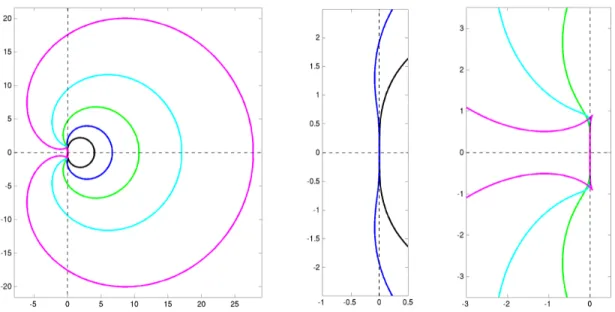
1.1 A(α)-stability (left) and stiff stability (right) takes place provided the shaded area is contained in the stability region of the ODE scheme. . . 11 1.2 A domain Ωgiven by the union of a disk Ω1 and a rectangle Ω2. . . 19 2.1 The left pane shows a plot of the boundaries of the regions of absolute

stability for all BDF methods of orders s = 2, . . . ,6. From innermost to outermost, the curves correspond to the methods of increasing order s. The regions of absolute stability are exterior to the corresponding boundaries. The middle (resp. right) pane shows a close-up near the origin of the boundaries for the methods of orders = 2,3(resp. s= 4,5,6). 28 2.2 The stability region of a hypothetical quasi-unconditionally stable method

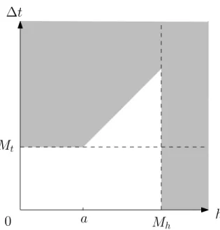
is shown in white in the parameter space (h,∆t). The grey region is the set of h and ∆t where the method is unstable. Notice that outside of this window in the region a < h < Mh and ∆t > Mt, the method is sta- ble for time steps satisfying the condition ∆t < h. Quasi-unconditional stability does not exclude the possibility of other stability constraints outside of the rectangular region of stability. . . 46

2.3 Demonstration of a CFL-like stability constraint when ∆t is outside the rectangular window of quasi-unconditional stability for the advection- diffusion equation with α = 1.0 and β = 0.05 (parameters selected for clarity of visualization. Theoretical value: Mt= 0.0965for this selection of physical parameters). The eigenvalues multiplied by ∆t (black dots) are plotted together with the boundary of the BDF5 stability region (dashed grey curve; cf. Figure 2.1). (a) Using N + 1 = 9 grid points and time step ∆t = 0.23 all eigenvalues lie within the stability region.

(b) The number of points is increased toN+ 1 = 19while the time step is held constant. The ten additional eigenvalues are not in the stability region, which indicates the method is unstable for these parameter val- ues. (c) The number of points is again N + 1 = 19, but the time step is reduced to ∆t = 0.12, causing all eigenvalues to be contained in the stability region. . . 78 2.4 Continuation of Figure 2.3. (a) The time step is ∆t = 0.12 (as in

Figure 2.3(c)) and the number of grid points is increased toN+ 1 = 35.

Once again, some eigenvalues do not lie in the stability region. (b) The number of grid points is held at N + 1 = 35 while the time step is reduced to ∆t = Mt = 0.0965, which is the maximum allowed for the window of quasi-unconditional stability. All eigenvalues now lie in the stability region. (c) With ∆t = 0.0965, additional eigenvalues (arising from further increasing the number of grid points) remain within the stability region, thus demonstrating the quasi-unconditional stability of the BDF scheme of order 5. . . 79 2.5 Maximum stable ∆t versus spatial mesh size h for Fourier-based BDF

and AB methods of orders three and four when applied to the advection- diffusion equation (2.115), with α= 1, β = 10⁻² on the left and α = 1, β = 10⁻² on the right. . . 80

2.6 Maximum stable ∆t versus spatial mesh size h for Fourier-based BDF and AB methods of orders three and four when applied to the advection- diffusion equation (2.115), with α= 1, β = 10⁻³ on the left and α = 1, β = 10⁻⁴ on the right. . . 81 3.1 Illustration of the FC(Gram) method, showing the original function val-

ues on the b-periodic domain (solid circles) together with the continua- tion values (open circles) which are obtained by summing the left and right blend-to-zero extensions (thin gray lines). The thick black curves indicate the polynomial approximations in the fringe regions which are used to produce the blend-to-zero extensions. . . 96 3.2 Numerical solution of the advection equation (3.4) at time t = 15 us-

ing second order finite differences (top), fourth order compact schemes (middle), and Fourier continuation (bottom). The numerical dispersion in the finite difference solutions is clearly visible at this solution time. . 98 3.3 One dimensional spatial convergence test of the variable coefficient FC-

ODE solver for the system (3.10) with exact solution (3.11). . . 101 3.4 One dimensional illustration of exchange boundaries. a)Domains 1 and

2 overlap perfectly in a region four points wide. b) At the data-passing step of the algorithm, the solution values of the last two points in each domain are substituted by the corresponding values in the neighboring subpatch. . . 107 4.1 Convergence of the two-dimensional BDF-ADI solvers of orders s =

2, . . . ,6 in a Cartesian square. . . 118 4.2 Convergence of the three-dimensional BDF-ADI solvers of orders s =

2, . . . ,6 in a Cartesian cube. . . 119 4.3 Convergence of the BDF2 ADI solver in an annulus with various mesh

discretizations and Reynolds numbers. . . 121

4.4 Convergence of the BDF3 ADI solver in an annulus with various mesh discretizations and Reynolds numbers. . . 121 4.5 Schematic set-up of unsteady flow over a bumpy plate (not to scale). . 122 4.6 Vertical velocity in two-dimensional boundary layer flow over a bumpy

plate, showing the presence of vortices and acoustic waves. From top to bottom, the solution times for the figures are t= 9.76, 9.82, 9.88, 9.94. 124 4.7 Geometry of Taylor-Couette flow. The fluid is confined to the region

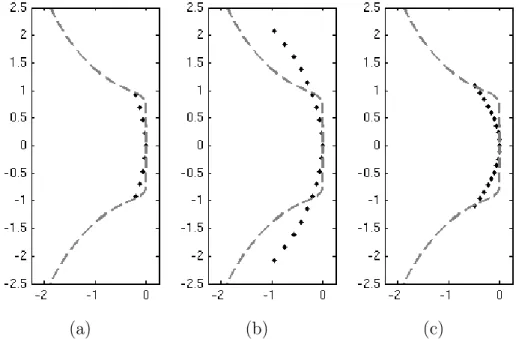
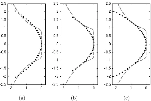
between two cylinders of radii ri and ro, and two planes separated by a length h. The inner cylinder rotates with speed Ui, while all other boundaries remain stationary. . . 126 4.8 Profiles of the (a) azimuthal velocity, (b) vertical velocity, and (c) az-

imuthal component of vorticity in small-aspect-ratio Taylor-Couette flow at Ma = 0.2 and Re = 700. The top (bottom) row has the profiles of the two-cell (one-cell) stable mode. . . 127 4.9 Two close-ups of the mesh used in the numerical experiments of flow

past a cylinder. The bottom figure shows the clustering of points near the cylinder surface to spatially resolve the boundary layer. . . 129 4.10 Temporal convergence of the solver for flow past a cylinder at time t =

1.0, withRe = 200 and Ma = 0.8. . . 131 4.11 Snapshot of the vorticity in a simulation of flow past a cylinder with

Re = 200, Ma = 0.2at time t= 82.8. . . 133 4.12 Time evolution of streamlines in flow past a cylinder at Re = 200 and

Ma = 0.2. Darker shading of the streamline corresponds to a higher magnitude of the velocity at that point. . . 134 4.13 Temporal convergence of the three-dimensional multi-domain solver us-

ing the method of manufactured solutions at timet = 1.0, withRe = 500 and Ma = 0.8. . . 135

4.14 Two-dimensional slice of the mesh for flow past a sphere. The coloring shows the sub-patch decomposition. . . 136 4.15 Two-dimensionalx-z slice of the streamlines in a simulation of flow past

a sphere with Re = 500, Ma = 0.5at time t = 12. Darker shades in the streamlines indicate higher velocity magnitude. . . 136 4.16 Two-dimensional x-z slice of the x-velocity (top) and density (bottom)

in flow past a sphere at Re = 500 and Ma = 0.5. . . 137 4.17 Isosurfaces of the density (ρ = 0.95) in three-dimensional flow past a

sphere at times t = 64.5 (top) and t = 77.5 (bottom), showing the apperance of hairpin vortices in the flow field. . . 138 B.1 Left: The “Yin” mesh with coarser grid spacing than used in the numer-

ical examples of flow past a sphere. Right: The composite “Yin-Yang”

mesh. . . 146

List of Tables

2.1 Coefficients for BDF methods of orders s = 1, . . . ,6. . . 29 2.2 Leading order term for the real part of z(θ), the boundary locus of the

BDF method of order s stability region as θ→0. . . 73 2.3 Numerical estimate of the constant mC such that for all m < mC

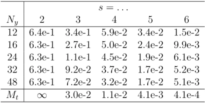
the parabola Γm described in Lemma 2.3 is contained in the region of absolute stability of the BDF method of order s. By Theorem 2.4, the order-s BDF method applied to the advection-diffusion equation ut+α ux =β uxx with Fourier collocation is stable for all∆t < _α^β2mC . 74 2.4 Maximum stable ∆t for BDF-ADI methods of orders s = 2, . . . ,6 at

Reynolds number Re = 10² and Mach number 0.9 in 2D with various numbers Ny of discretization points in the y variable. The number of discretization points in the x direction is fixed at Nx = 12. The con- stant Mt of quasi-unconditional stability predicted by the linear theory (equation (2.127)) is given in the last row. . . 85 2.5 Same as Table 2.4 but with Reynolds number Re = 10³. . . 85 2.6 Same as Table 2.4 but with Reynolds number Re = 10⁴. A “Q” in the

table means there was no stable ∆t found for the given discretization.

However, using 16 points in the x direction, all entries in the table can be filled, which is an indication of the quasi-unconditional stability of the method. . . 85 3.1 Coefficients for AB methods of orders s= 1, . . . ,4. . . 105

3.2 Number of seconds S needed per processor for the parallel implicit al- gorithm to advance one million unknowns forward one time step, with various numbers of discretization points, sub-domains, and subiterations. 115 4.1 Parameters for two-dimensional manufactured solution. The temporal

frequencies λj not in parentheses are the ones used in the convergence tests for the methods of orders s = 2,3, while the ones in parentheses are those used in the order s= 4,5,6 tests. . . 120 4.2 Parameters for three-dimensional manufactured solution. The temporal

frequencies λj not in parentheses are the ones used in the convergence tests for the methods of orders s = 2,3, while the ones in parentheses are those used in the order s= 4,5,6 tests. . . 120

Chapter 1 Introduction

The direct numerical simulation of fluid flow at high Reynolds numbers presents a number of significant challenges—including the presence of structures such as bound- ary layers, eddies, vortices and turbulence, whose accurate spatial discretization re- quires use of fine spatial meshes. CFD (computational fluid dynamics) simulation of such flows by means of explicit solvers is highly demanding, even on massively parallel super computers, in view of the severe restrictions on time steps required for stability:

the time step must scale like the square of the spatial mesh size. Classical implicit solvers do not suffer from such time step restrictions but they do require solution of large systems of equations at each time step, and they can therefore be extremely expensive as well.

The celebrated Beam and Warming method [6, 8] provides one of the most attrac- tive alternatives to explicit and classical implicit algorithms. Based on the alternating direction implicit method [69] (ADI), the Beam and Warming scheme enables stable solution of the compressible Navier-Stokes equations in times that grow only linearly with the size of the underlying discretization, and without recourse to either nonlinear iterative solvers or solutions of large linear systems at each time step. As discussed in detail in the introductory portion of Chapter 2, however, previous work in the context of the Beam and Warming method has not demonstrated accuracies beyond the first order of temporal accuracy.

Nevertheless, high-order time accuracy may be crucial in the treatment of long- time simulations or highly-inhomogeneous flows—for which the dispersion inherent in low-order approaches would make it necessary to use inordinately small time-steps.

This thesis presents, in particular, extensions of the ADI methodology based on the backward differentiation formulae (BDF) that exhibitorders of time accuracy between two and six, and which are quasi-unconditionally stable, in a sense that is made clear in Section 2.2—which essentially amounts to true unconditional stability within certain regions in the space of discretization parameters. Further, full unconditional stability of the second order scheme is established in the context of the convection and parabolic linear equations. An extended discussion is presented in this thesis which places on a solid theoretical basis the observed quasi-unconditional stability of the s order methods with 2≤s≤6. In fact this thesis presents, for the first time in the literature, high-order time-convergence curves for Navier-Stokes solvers based on the ADI strategy.

The proposed methodology employs the BDF schemes (which are known for their robust stability properties) together with a quasiliner-like formulation with high- order extrapolation for nonlinear components (to produce a linear high-order time- accurate method) and the Douglas-Gunn splitting (an ADI strategy that greatly simplifies boundary condition treatment while retaining the order of time-accuracy of the solver). The performance of the proposed solvers is favorable: for example, a two- dimensional rough-surface configuration including boundary layer effects at Reynolds number 10⁶ and Mach number Ma = 0.8 (with a well-resolved boundary layer, run up to a sufficiently long time that single vortices travel the entire spatial extent L of the domain, and with spatial mesh sizes near the wall of the order of 10⁻⁵ ·L) was successfully tackled in a relatively short (∼ thirty-hour) single-core run; under similar circumstances an explicit solver would require truly prohibitive computing times. The highest order solvers can be greatly advantageous for problems involving long evolution times or solutions that oscillate rapidly in time; methods of lower order

may be more advantageous under other circumstances.

While the computational cost of the proposed BDF-ADI schemes mentioned above grows only linearly with the size of the spatial discretization, these schemes are sig- nificantly more expensive per time step than their explicit counterparts—such as the explicit Fourier Continuation solver [2] (FC) we use. Thus the strategy pro- posed in this thesis calls for use of multi-domain implicit-explicit solvers—implicit near boundaries and other regions where fine spatial discretizations are used (which might require extremely small time steps in an explicit solver), and explicit in re- gions in which the size of the spatial discretization does not entail significant CFL constraints. (The proposed multi-domain implicit-explicit schemes should not be con- fused with similarly named IMEX methods [4] which, e.g., in an advection-diffusion equation incorporate explicit treatment of the convective term and implicit treatment of the diffusive term.) A brief description of the Fourier continuation methodology and associated explicit solvers is presented below followed by an outline of the pro- posed multi-domain implicit-explicit strategy; complete descriptions and illustrations of these solvers follow as part of the main body of this thesis.

Most structured-grid solvers for Partial Differential Equations (PDE) are based on the use of finite differences (FD). These methods are intuitively attractive, they can be implemented easily, and they require limited cost per spatial discretization point.

As is well known, however, reduction of the dispersion error inherent in FD methods requires either use of large numbers of points per wavelength, or use of higher-order methods which typically entail higher costs and restrictive CFL constraints [2, 3, 35].

Spectral methods are an attractive alternative in dealing with these challenges [10, 19, 47]. Unfortunately, polynomial spectral methods require clustering of points at the boundaries of the domain, resulting in severe time step restrictions for explicit methods. Classical Fourier methods, on the other hand, are only applicable to periodic problems—otherwise they suffer from the Gibbs phenomenon and first order spatial convergence in the interior of the domain (see, e.g., [10, Ch. 2.2]). The recently

introduced Fourier Continuation method (FC) provides spectral-like resolution in non-periodic contexts without recourse to use of fine meshes; we briefly discuss this methodology in what follows.

The FC method produces an interpolating Fourier series representation by relying on a “periodic extension” of a given function, that closely approximates it in the physical domain, but which is periodic on a slightly enlarged domain. In the context of explicit algorithms, following [2, 3, 35] the FC spatial discretizations are used in conjunction with the Adams-Bashforth (AB) method [58, Ch. 3.9] of orders two through four. As shown in Section 3.1.2 as well as in previous references [2, 3, 35, 64], the resulting FC time-domain solvers (whether explicit or implicit) do give rise to significantly improved dispersion properties, low computing costs, high accuracies and favorable spectral asymptotics in CFL constraints—as well as parallelization with perfect scaling. In particular, the explicit solver is significantly more accurate than other explicit methods for similar computing times, and significantly faster than other schemes for a given accuracy; cf. [2] and Section 3.1.2.

Unlike previous general Navier-Stokes solvers, all of the methods presented in this thesis, including the explicit, implicit, and multi-domain solvers mentioned above, enjoynear spatial dispersionlessnessas well ashigher orders of accuracy in both space and time. Such desirable characteristics are demonstrated, in particular, by means of implicit solutions in single domains as well as explicit and multi-domain implicit- explicit solutions with non-trivial boundary conditions—all of which include no-slip boundary conditions at walls, and, depending on the case under consideration, ab- sorbing boundary conditions and inflow conditions. The proposed BDF-ADI solvers, further, enjoy both the properties of quasi-unconditional stability, dispersionlessness, and high-order accuracy in time. The multi-domain implicit-explicit solver, in turn, is highly effective: results of two-dimensional flow past a cylinder and three-dimensional flow past a sphere were produced with a significant cost savings over purely explicit or implicit solvers. These results also represent the first demonstrations of high-order

time-accuracy for any Navier-Stokes solver with an implicit component (let alone any hybrid solver) in flows of physical interest. In view of a variety of numerical examples presented in this thesis we suggest that the accuracy levels achieved by the proposed solvers for given spatial and temporal discretizations are unprecedented in the literature.

In the remainder of this chapter we provide a brief account of the background leading to the contributions in this thesis. The proposed BDF-ADI solvers are then introduced in Chapter 2, including the concept of quasi-unconditional stability as well as energy stability proofs for the second order schemes and spectral stability proofs for the higher-order BDF methods. The multi-domain implicit-explicit schemes are then presented in Chapter 3. Numerical results follow in Chapter 4, and concluding remarks, finally, are presented in Chapter 5.

1.1 The Navier-Stokes equations for a compressible gas

We consider the Navier-Stokes equations for a continuum fluid. Denoting by _Dt^D =

∂

∂t +u· ∇ the material derivative, the Navier-Stokes system combines the equations describing conservation of mass,

Dρ

Dt +ρ∇ ·u = 0, (1.1)

conservation of momentum,

ρDu

Dt +∇p=∇ ·σ, (1.2)

and conservation of energy, ρDe

Dt +p∇ ·u+∇ ·q = Φ, (1.3)

where d denotes the spatial dimensions (d = 2, 3) and where, using integer-valued indices i, j = 1, . . . , d, u = (ui) denotes the velocity vector, and ρ, e, p, q,σ = (σij), and Φ = P

ijσij∂xiuj denote density, specific internal energy, pressure, heat flux, deviatoric stress tensor, and viscous dissipation function, respectively. We narrow our consideration to the evolution of a subsonic compressible perfect gas satisfying the following assumptions:

1. The fluid is Newtonian, i.e., σ = µ ∇u+∇u^T − ²₃(∇ ·u)I

, where µ is the viscosity and Iis the identity tensor.

2. The internal energy and temperature T satisfy the thermodynamic relation e=cvT, where cv is the specific heat at constant volume.

3. The pressure, density, and temperature are related by the equation of state for an ideal gas p=ρRT, where R is the gas constant.

4. Fourier’s law of heat conduction q = −κ∇T holds, where κ is the thermal conductivity.

5. For simplicity, µand κ are functions of temperature only.

With these assumptions, choosing a characteristic length L0, velocity u0, density ρ0, temperature T0, viscosity µ0, and heat conductivity κ0, and with a slight notational abuse by which the non-dimensional density, velocity, and temperature ρ/ρ0, u/u0, and T /T0 are denoted everywhere below in this thesis by the symbols ρ, u, and T, respectively, the non-dimensional form of the Navier-Stokes equations

ρt+∇ ·(ρu) = 0 (1.4a)

ut+u· ∇u+ 1 γMa²

1

ρ∇(ρT) = 1 Re

1

ρ∇ ·σ (1.4b)

Tt+u· ∇T + (γ−1)T∇ ·u = γ RePr

1

ρ∇ ·(κ∇T) + γ(γ−1)Ma² Re

1

ρΦ (1.4c)

results, where the non-dimensional constants γ = cp/cv, Re = ρ0u0L0/µ0, Ma = u0/√

γRT0 andPr =µ0cp/κ0 denote the ratio of specific heats, the Reynolds number, the Mach number and the Prandtl number, respectively.

The system is completed by means of the relevant boundary conditions for a given configuration; see, e.g., [95, Sec. 1-4] and Remark 2.1.

1.2 Implicit solvers

This section provides a brief overview of the history of implicit methods, including considerations ofstability and accuracy. Section 1.3 then discusses one of the highly significant innovations concerning efficiency in implicit methods, namely, the alter- nating direction implicit strategy.

1.2.1 Stability and convergence

The 1928 landmark paper by Courant, Friedrichs and Lewy [23] established that a consistent numerical method need not converge to the exact solution of the corre- sponding PDE, even though the numerical approximation of the problem is arbitrarily accurate. Specifically, that paper showed that the centered difference scheme for the wave equation cannot converge for general initial conditions unless the numerical do- main of dependence includes the physical domain of dependence. This leads to a linear constraint (the CFL constraint) of the form

∆t≤C h

for the time step∆tand the spatial mesh sizeh. Note that the result is only concerned with convergence—it does not indicate what happens to a non-converging numerical solution of a consistent scheme. It was not until Lax’s equivalence theorem [59] in the 1950s that the connection with stability was made clear: any consistent numerical

method for a linear PDE converges if and only if it is stable. Certainly, while not the name itself, the concept of stability does predate this contribution. For example, Crank and Nicolson presented in the 1947 paper [24] the first implicit method for PDEs based on the trapezoidal rule for time integration and showed (using a sugges- tion by von Neumann communicated to those authors by Hartree) that the method was stable for the heat equation for all grid spacingshand time steps∆t, whereas the leapfrog scheme (“Richardson’s method”) was not. However, the word “stable” in any form does not appear in the article—what is now known as instability was termed

“rapidly increasing oscillatory error” in that early contribution.

In 1956 Dahlquist [26] established a convergence theorem for the numerical solu- tion of ordinary differential equations (ODE) with linear multistep methods, which is similar in spirit to Lax’s equivalence theorem (in the later contribution [27] Dahlquist mentions, “When I wrote [that paper], I was not yet familiar with the work of Lax”).

Dahlquist’s result is as follows: given an ODE of the form y⁰ =f(y, t), y(0) =y0,

where the function f(y, t) satisfies certain Lipschitz conditions, a linear multistep method for the ODE, given by a formula of the form

s

X

j=0

ajy^n+j = ∆t

s

X

j=0

bjf^n+j (1.5)

for some coefficients aj and bj, converges if and only if the method is stable for the ODE y⁰ = 0 (i.e., the method iszero-stable).

As a consequence of these results the stability of a scheme takes absolute prece- dence over considerations of accuracy. The challenges arising from stability con- straints in practical applications became painfully clear with the consideration of

“stiff” differential equations, a term first used by Curtiss and Hirschfelder in [25].

In stiff problems the stability constraint requires use of time steps that are much

smaller than is otherwise necessary to resolve the time evolution of the problem. The contribution [25] also introduces what would later become known as the backward differentiation formulae (BDF) multistep methods as a remedy for this difficulty, and thereby demonstrates the great value of the unconditional stability property that is sometimes afforded by implicit methods for solutions of stiff differential equations.

Unfortunately, soon after this was established, certain severe limitations of implicit methods in terms of temporal accuracy order were soon discovered, as discussed in the following section.

1.2.2 Order barriers

Consider the test problem

y⁰(t) = λy(t) (1.6)

with λ in the complex plane C, together with an associated numerical scheme and a given time step ∆t; as is known, any linear multistep numerical method for equa- tion (1.6) can be expressed in terms of the quantity z =λ∆t. LettingR ⊆C denote the set ofz =λ∆tfor which the scheme is stable when applied to the above equation, the question thus arises as to whether the scheme is “optimally” stable in this context, that is, whether it is stable for all ∆t and for all λ for which the ODE solution is asymptotically stable as t→+∞. Or, equivalently, since (1.6) is asymptotically sta- ble for for all complex values λ in the set C⁻ of complex numbers with non-positive real part, the question becomes whether the numerical scheme is stable for allz ∈C⁻. A method satisfying this condition is said to be A-stable. For stiff problems, which include spectral components of the form (1.6) with large magnitude values ofλ ∈C⁻, the value of A-stable methods is unquestionable.

Unfortunately, however, a fundamental limit to the accuracy order of A-stable methods is imposed by Dahlquist’s second barrier: There are no A-stable explicit linear multistep methods, and an (implicit) A-stable linear multistep method has ac-

curacy order not higher than two. There have been many attempts to “break” this barrier by considering more general classes of multistep methods; see, e.g., the meth- ods surveyed in [46, Chap. V.3]. There are also higher-order implicit Runge-Kutta methods, which are not covered by Dahlquist’s theorem. Nevertheless, all such meth- ods are subject to a more general result—the Daniel-Moore conjecture [29], proved in [93]—which demands that higher-order A-stability comes at the cost of a certain number of implicit solves. Specifically, any A-stable Runge-Kutta or generalized mul- tistep method with a number s of implicit stages can have time accuracy not higher than 2s.

Given that the use of methods that include s implicit steps can be exceedingly expensive in the PDE context (cf. the discussion in Section 3.5.2 concerning even a single fully-dimensional implicit solve), the alternative is to consider higher-order methods which, while not A-stable, admit useful stability regions. In the language of this thesis, higher-order multistep methods for the Navier-Stokes equations and other PDEs do exist, namely quasi-unconditionally stable methods, which enjoy favorable stability restrictions.

1.2.3 Higher order implicit methods: ODE theory

Following Dahlquist’s landmark 1963 contribution [28], a number of attempts were made to identify and study classes of ODE solvers with favorable stability properties.

Two important concepts, namely, A(α)-stability and stiff stability, arose from these efforts. A method is said to be A(α)-stable if the stability region R contains the infinite “α-wedge” with vertex at the origin, given by{z| arg(z)∈(π−α, π+α), z6= 0}. A method is stiffly stable if the stability region includes the semi-infinite region {z|Rez <−a}as well as the rectangle {z|Rez ∈(−a,0), Imz ∈(−c, c)}for positive numbers a and c. Both of these concepts are illustrated in Figure 1.1.

Unfortunately, these definitions do not provide the level of detail necessary to ad- equately discuss the stability of PDEs such as the Navier-Stokes equations amongst

α α

i c

− i c

− a

Figure 1.1: A(α)-stability (left) and stiff stability (right) takes place provided the shaded area is contained in the stability region of the ODE scheme.

many others. To demonstrate this difficulty we consider the advection-diffusion equa- tion

ut+αux =βuxx, (1.7)

which is undoubtedly the simplest model problem that could be used to understand basic aspects of the Navier-Stokes equation. As will be shown in Section 2.4, the eigenvalues associated with the multistep schemes for this equation are distributed in curves that are not contained in anyα-wedge with α < π/2; cf. Figure 1.1.

The concept of stiff stability, on the other hand, is not well suited for discussion of the PDEs under consideration, since the stiff-stability regions, which are bounded by vertical and horizontal lines, can only provide relatively crude bounds on the parabolic-bounded eigenvalue distributions for the types of PDEs under considera- tion. In fact, the BDF stability regions, which approximate more closely the PDE eigenvalue distributions and which provide highly stable algorithms, are not stiffly stable in some cases. Additionally, considerations based on stiff stability might sug- gest that the fifth and sixth order BDF-ADI methods proposed in this work, which are stiffly stable, ought to give rise to better stability properties in practice than the corresponding BDF-ADI methods of orders three and four, which are not stiffly sta- ble. This suggestion is not accurate, however. In practice, and as shown rigorously in

Section 2.4 for the linear advection-diffusion equation, the BDF-ADI methods of or- ders three and four are stable for a significantly larger set of discretization parameters than those required for stability in the methods of orders five and six.

We thus see that some of the concepts from ODE theory are not well adapted to the context of the PDE under consideration—at least for methods of order higher than two. (In contrast, the concept of quasi-unconditional stability introduced in Section 2.2 does accurately capture the stability character of the BDF-ADI methods proposed in this thesis.) Additionally, as discussed in the following section, implicit methods with orders of temporal accuracy higher than two have received only sparse attention in the literature. Thus the goal of the present thesis: to provide temporally high-order Navier-Stokes solvers with unconditional stability or, failing that, with as close a substitute as possible.

1.2.4 Higher order implicit methods: PDE applications

The state of the art for solvers of compressible flow is second order time accuracy as far as implicit methods are concerned—and, indeed, we believe second or higher order time-accuracy for general domains and boundary conditions has not been demon- strated before this work. The most significant innovations for compressible fluid solvers have concerned implementation techniques that improve efficiency (e.g., opera- tor splittings and multigrid) orrelative accuracy (e.g., Newton-like subiterations), but such improvements do not increase the order of accuracy of the underlying method.

Perhaps the existence of Dahlquist’s second barrier may explain the widespread use of implicit methods of orders less than or equal to two (such as backward Euler, the trapezoidal rule and BDF2, all of which are A-stable), and the virtual absence of implicit methods of orders higher than two—despite the near-universality of the fourth order Runge-Kutta and Adams-Bashforth explicit counterparts. Clearly, A- stability is not necessary for all problems—for example, any method whose stability region contains the negative real axis (such as the BDF methods of orders two to six)

generally results in an unconditionally stable solver for the heat equation. A number of important questions thus arise: Do the compressible Navier-Stokes equations in- herently require A-stability? Are the stability constraints of all higher-order implicit methods too stringent to be useful in the Navier-Stokes context? How close to un- conditionally stable can a Navier-Stokes solver be whose temporal order of accuracy is higher than two?

Unfortunately, clear answers to these questions are not available in the literature.

For example, the 2002 reference [9] compares various implicit methods for the Navier- Stokes equations, and it states: “Practical experience indicates that large-scale engi- neering computations are seldom stable if run with BDF4. The BDF3 scheme, with its smaller regions of instability, is often stable but diverges for certain problems and some spatial operators. Thus, a reasonable practitioner might use the BDF2 scheme exclusively for large-scale computations.” However, the paper and references therein do not investigate the stability restrictions for the higher-order BDF methods, either theoretically or experimentally. As abundantly demonstrated in Chapter 4, however, methods of order higher than two can have very significant advantages for certain classes of problems, and thus, it seems useful to make available methods of a variety of temporal orders, each one of which may be best adapted to corresponding classes of subproblems—say, to high-frequency or to low-frequency problems; to problems requiring solutions for small times or to problems requiring solution for long times, etc.

The recent 2015 article [37], in turn, presents applications of the BDF scheme up to third order of time accuracy in a finite element context for the incompress- ible Navier-Stokes equations with turbulence modelling. This contribution does not discuss stability restrictions for the third order solver, and, in fact, it only presents nu- merical examples resulting from use of BDF1 and BDF2. The 2010 contribution [53], which considers a three-dimensional advection-diffusion equation, presents various ADI-type schemes, one of which is based on BDF3. The BDF3 stability analysis in

this paper, however, is restricted to the purely diffusive case.

The above examples illustrate the need for theoretical analyses and numerical investigations of higher-order implicit methods for PDEs. A major goal of this thesis is to make progress on both of these fronts, thus laying the groundwork for further work in this area.

1.3 Alternating direction implicit methods

ADI methods are based on a certain operator splitting technique (in fact, the first such technique ever introduced): they tackle PDE problems by “splitting” the relevant underlying operator, giving rise to relatively simpler problems. In the context of a first order system of PDEs ut = Lu, for example, operator splitting techniques use expressions of the operator L as the sum of two or more operators, L = P

jLj, which describe different characteristics of the problem. For example, the splitting may be along the lines of slow and fast processes, small and large scales, advective and diffusive terms, linear and nonlinear terms, or, as in the case of the ADI methods, derivatives in each spatial dimension.

The first ADI methods were introduced in the landmark papers by Peaceman and Rachford [69] and Douglas [30], where the schemes were used to solve the heat equation in two dimensions,

ut=uxx+uyy.

Using a time step ∆t, and centered finite difference approximations δxx and δyy for the second order derivatives, the Peaceman-Rachford scheme for the approximate solutionuⁿ⁺¹ at timet = (n+ 1)∆t (for non-negative integer n) can be written as

(I −∆t δxx)u^∗ = (I+ ∆t δyy)uⁿ (I−∆t δyy)uⁿ⁺¹ = (I+ ∆t δxx)u^∗,

which is formally second order accurate in space and time. Thus, the ADI split- ting turns a large sparse system of equations into two sets of one-dimensional equa- tions which can be solved efficiently with tridiagonal algorithms, greatly reducing the time and memory requirements previously needed by implicit methods for multi- dimensional PDEs.

The original papers [30, 69] generated much interest in the ADI approach, giving rise to a number of early contributions on the subject, such as the works of Douglas and Gunn [31, 32], Fairweather and Mitchell [36], D’Yakonov [33], and Yanenko [96].

Applications to problems of fluid dynamics began with the works of Pearson [70] and Chorin [22] for the incompressible Navier-Stokes equations. Briley and McDonald [11]

developed ADI schemes for the compressible Navier-Stokes and Euler equations.

Undoubtedly, the best-known ADI schemes for compressible fluid-dynamics are the methods of Beam and Warming [6, 8] (also known as approximate factorization methods (AF)), which have been successfully used for years in many compressible Navier-Stokes solvers, e.g., [34, 41, 54, 72, 89, 90]. Besides the advantages gained by using the ADI methodology, the Beam and Warming method also enjoys other at- tractive properties: The time discretization is cleverly chosen in such a way that the stability of the scheme (for certain two dimensional linear problems) follows imme- diately from the stability for the underlying one-dimensional multistep method [94].

The method does use a linearization strategy based on first-order Taylor expansion of certain nonlinear fluxes, which is consistent with the nominally second-order temporal accuracies inherent in the underlying time-stepping schemes used.

Despite the success of ADI methods in general and the Beam and Warming method in particular, challenges have remained. For example, the linearization strategy based on the Taylor expansion mentioned above cannot be used in a higher-order method (since higher order terms necessarily give rise to nonlinearities). The stability of ADI methods is also difficult to analyze and, indeed, it is known [94] that the Beam and Warming method is unstable for three dimensional linear advection equations,

although it is unconditionally stable in the two dimensional advection case.

Significant follow-up efforts [34, 41, 54, 72, 89, 90] have centered around the ideas first put forth in the celebrated papers [6, 8], focusing, in particular, on enhancing stability and restoring the (nominal) second order of accuracy inherent in the original derivation of the method. The aforementioned follow-up algorithms incorporate vari- ous kinds of Newton-like subiterations to reduce the errors arising from the nonlinear terms while maintaining stability. In spite of these additions, however, the follow-up contributions still do not demonstrate second order accuracy in time by means of numerical examples—even though in all such cases nominally second order time step- ping schemes are used. In contrast, these contributions do demonstrate the expected spatial order of accuracy with a variety of numerical examples.

Perhaps the lack of numerical evidence for second-order accuracy of the Beam and Warming method can be attributed to one of the most persistent challenges for ADI schemes—namely, the prescription of boundary conditions for intermediate unknowns that are stable and do not degrade the order of accuracy of the scheme (see, e.g., the discussions in [10, Ch. 13.3] and Section 2.1.5). Although methods can sometimes be derived for simple Dirichlet conditions (such as the boundary treatment proposed by Beam and Warming in [7] for a scalar parabolic equation), they cannot be applied to more general boundary conditions. Many attempts have been made to overcome this difficulty; for example, the contribution [77] proposes a general finite difference boundary treatment for the intermediate steps of the Beam and Warming method, but the numerical experiments do not show second order convergence of the scheme.

Furthermore, the authors note the following:

“Beam and Warming indicated that the implicit factored method employed in the present study should be unconditionally stable. Nevertheless, in- stability occurs when the time step size exceeds a certain limit. Numerical experiments performed here showed that for the conditions of the present study, the solution was always stable when the time step size (∆t) satisfied

the expression

∆t <60∆W/a0.

∆W is the smallest grid size employed in the study and a0, is the speed of sound.”

It is unclear whether the CFL stability constraint is due to the boundary treatment or the Beam and Warming method itself.

The boundary condition difficulties that exist for many ADI schemes can usu- ally be traced back to a simple fact: the intermediate unknowns that arise from the splitting are not necessarily consistent approximations of the physical solution.

A notable exception in this regard is the splitting procedure developed by Douglas and Gunn [32]. Although not mentioned in the original papers, it was later under- stood [12] that the Douglas-Gunn splitting (with formal order of accuracy s = 2) yields equations for the intermediate unknowns that approximate the original PDE to order s−1 = 1. It follows that using the physical boundary conditions attⁿ⁺¹ for the intermediate steps preserves the order of accuracy of the method.

This thesis proposes ADI methods that address and overcome all the extant chal- lenges to ADI-based solvers. The underlying BDF multistep method together with BDF-like extrapolation for the nonlinear terms provides higher-order-accurate meth- ods with quasi-unconditional stability. An extension of the Douglas-Gunn splitting to our context guarantees the correct order of accuracy even in the presence of general boundary conditions.

1.4 Domain decomposition

Without question, a necessary component of any solver for the challenging problems in CFD is a method of domain decomposition. The advantages are twofold: 1) The decomposition provides a covering of the global solution domain with simpler sub- domains on which an approximate solution can more easily be computed and 2) a

domain decomposition is the natural basis for dividing the computational workload in a parallel implementation of a numerical solver. In this section we give a brief history of some domain decomposition strategies relevant to the one presented in this thesis.

1.4.1 The Schwarz alternating method

The earliest contribution to domain decompositions for partial differential equations is also the foundation of most modern domain decomposition solution strategies—

namely, the Schwarz method [75] which Schwarz developed for the same reason as given in point 1) in the introduction to this section—to solve a problem on a complex domain by using known solution methods on simpler ones. Here we give a brief history of the Schwarz method; see [40] for a more detailed account.

In his Ph.D. thesis, Riemann had taken for granted the existence of solutions to Laplace’s equation in general domains when he proved what would later be known as the Riemann mapping theorem. When it came to his attention, he invoked what is now called Dirichlet’s principle—that the solution of Laplace’s equation in a domainΩ with u=g on the boundary is given by the minimizer of the non-negative functional

J(u) = Z

Ω

1 2∇u²

among all twice-differentiable usatisfying the boundary conditions. However, Weier- strass showed with a counterexample that a non-negative functional need not attain a minimizer. Of course, the existence of harmonic functions was established for simple domains, like disks and rectangles. Schwarz used this fact to construct solutions in more complex geometries.

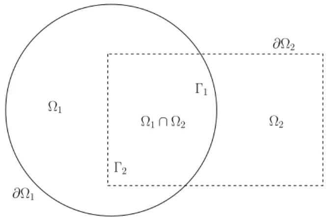
Ω₁

Ω₁∩Ω₂ Ω₂

Γ₂

Γ₁

∂Ω1

∂Ω2

Figure 1.2: A domain Ω given by the union of a diskΩ1 and a rectangle Ω2. For example, consider the problem

∆u= 0 inΩ u=g on∂Ω

where the domain Ω is given by the union of two sub-domains Ω1 and Ω2 such that Ω1 ∩Ω2 6= {∅}, as shown in Figure 1.2. (The disk and rectangle geometry is the example Schwarz himself used in his paper.) Let Γ1 =∂Ω1 ∩Ω2 and Γ2 =∂Ω2∩Ω1. The original Schwarz method produces the two sequences u^k₁ and u^k₂ given by the solutions of the sub-problems















∆u^k+1₁ = 0 in Ω1

u^k+1₁ =g on ∂Ω1∩∂Ω u^k+1₁ =u^k₂ on Γ1















∆u^k+1₂ = 0 inΩ2

u^k+1₂ =g on∂Ω2∩∂Ω u^k+1₂ =u^k+1₁ onΓ2.

(1.8)

This is also known as thealternating Schwarz method. Notice that the solution of the second problem requires the solution of the first, so that the procedure is sequential.

Convergence of this method follows, in essence, from the maximum principle for harmonic functions.

In the early 1990’s, Lions formally introduced theparallel Schwarz method in [63],

which is a modification of the original method (1.8) given by the sub-problems















∆u^k+1₁ = 0 in Ω1

u^k+1₁ =g on ∂Ω1\Γ1

u^k+1₁ =u^k₂ on Γ1















∆u^k+1₂ = 0 in Ω2

u^k+1₂ =g on ∂Ω2\Γ2

u^k+1₂ =u^k₁ on Γ2.

(1.9)

Notice that the problems are independent, and thus form the basis for an elliptic PDE solver in a distributed computing environment.

1.4.2 Overset/Chimera/composite grid methods

More than 20 years before the work of Lions, Volkov made the first application of the Schwarz method to fully discrete PDEs in the method of composite meshes [92]—

indeed, Section 8 of that paper is entitled “The use of Schwarz’s alternating method for solving a system of difference equations.” This was also the first instance of a general class of methods which were developed around the same time and under different names—the composite mesh method [79], the Chimera grid method [80], and the overset grid method [13] being among the most common. In this thesis, we will use the latter of these terms.

The overset grid method is ideally suited for solvers relying on spatial discretiza- tions that make use of structured grids. Briefly, it involves decomposing the physical domain into a set overlapping logical rectangles, whereby a sub-problem is solved on each of the constituent grids. Data is communicated between these component grids by means of interpolation.

After the introduction of the overset grid method by Volkov and subsequent de- velopment by Starius [79], applications to CFD problems were explored by Steger, Dougherty, and Benek [80]. The method reached a state of maturity in the 1990s with the development of general purpose grid generation software, such as CMPGRD [21], later to evolve into the object oriented suite Overture [13], which also includes basic

capabilities for solving certain PDEs on overset grids. Of course, all the early work on overset methods was done in the context of finite differences.

More recently, the overset grid strategy has been successfully developed with the FC methodology for the solution of the compressible Navier-Stokes equations in two dimensions [2] and the elasticity equations in three dimensions [3]. A key development in those contributions is the extension of the FC method to overlapping “sub-patch”

block-decompositions of larger meshes. Although the contributions [2,3] have success- fully used the overset method in the context of explicit solvers, the goal of extending the framework to implicit and multi-domain implicit-explicit solvers has not yet been fully realized until now. This thesis presents the first steps toward a general frame- work for the solution of time-domain problems using multi-domain implicit-explicit FC solvers.

1.5 Outline of this thesis

The general outline of this thesis is as follows:

Chapter 2 introduces the BDF-ADI solver for the Navier-Stokes equations. A de- tailed derivation is presented, which includes consideration of curvilinear coordinate systems, treatment of nonlinear terms, the Douglas-Gunn splitting technique, and handling of boundary conditions for the intermediate unknowns. The heart of this chapter is the rigorous mathematical framework that is developed in support of the BDF-ADI method. Rigorous energy proofs of unconditional stability for the Fourier- based BDF2-ADI scheme are given for two-dimensional linear advection and parabolic equations. The concept of quasi-unconditional stability is introduced, and we prove that the Fourier-based BDF methods of orders s = 2, . . . ,6 for the linear advection- diffusion equation in one, two, and three dimensions are quasi-unconditionally stable.

Finally, numerical investigations compare the stability of BDF schemes with explicit Adams-Bashforth methods, and quasi-unconditional stability is numerically demon-

strated for the BDF-ADI schemes applied to the full Navier-Stokes equations in two dimensions.

Chapter 3 presents the remaining elements necessary to complete the full multi- domain implicit-explicit solver. The Fourier continuation methodology is presented, together with examples showing its higher-order accuracy and dispersion relation pre- serving property. We review the explicit time marching used in the explicit zones of the multi-domain solver as well as the overset method and sub-patch domain decom- position strategies. The implicit-explicit time marching method is presented, and a simple example using the advection-diffusion equation in one dimension shows the convergence rate of the parallel time-marching method. Numerical performance stud- ies of the implicit multi-domain algorithm in a distributed computing environment are also documented.

Chapter 4 showcases the BDF-ADI and multi-domain solvers with a variety of numerical examples. The single domain BDF-ADI results use a Chebyshev collocation spatial discretization, demonstrating the stability of the solvers even in the face of very fine grid spacing. Numerical tests for this single-domain BDF-ADI solver include two dimensional unsteady flow over a bumpy plate at Reynolds number 10⁶ as well as three dimensional wall bounded Taylor-Couette flow. Subsequently, results of the implicit-explicit multi-domain solver in fully parallel simulations of two dimensional flow past a cylinder and three dimensional flow past a sphere are presented. In all cases, convergence studies are included that verify the expected temporal order of accuracy of the proposed solvers—a first for implicit Navier-Stokes solvers; limited emphasis is placed on the well understood [2,10,19,47]spatialhigh-order convergence and dispersionlessness of the methods used.

Chapter 2

BDF-ADI time marching method

This chapter introduces ADI solvers of higher orders of time accuracy (orderss= 2to 6) for the compressible Navier-Stokes equations in two- and three-dimensional curvi- linear domains. The new ADI algorithms successfully address the difficulties discussed in Section 1.3: (i) They (provably) enjoy high orders of time-accuracy (orders two to six)even in presence of general (and, in particular, non-periodic) boundary conditions;

and (ii) They possess remarkable stability properties, with rigorous unconditional- stability proofs for constant coefficient hyperbolic and parabolic equations for s = 2, and demonstrating in practice quasi-unconditional stability for 2 ≤ s ≤ 6 (Defini- tion 2.1) andmild CFL-like constraints outside the unconditional-stability window for s ≥ 3 (see Section 2.4.1); and (iii) They do not require use of iterative nonlinear solvers for accuracy or stability, and they rely, instead, on a BDF-like extrapolation technique for certain components of the nonlinear terms.

The algorithms presented in this chapter, which are based on a recently developed ADI algorithm for the two-dimensional nonlinear Burgers system [15], are applica- ble to generalsingle domain curvilinear coordinate systems and are restricted in this chapter to spectral spatial discretizations resulting from use of Fourier or polynomial spectral expansions; an accuracy order-preserving spectral filter is used in our scheme to ensure stability. Extensions of these algorithms to the multi-domain overset-grid context [13] as well as to the Fourier Continuation spatial discretization [2], are pre-

sented in subsequent chapters of this thesis. In particular, the present curvilinear domain algorithms form the single-domain implicit component of our general multi- domain implicit-explicit solver.

This chapter is organized as follows: Section 2.1 presents a derivation of the BDF-ADI method in two and three dimensions, starting with a quasilinear-like for- mulation of the equations and a transformation to general coordinates. The equation is then discretized in time using the BDF scheme and the treatment of nonlinearities by means of temporal extrapolation is presented. The resulting semi-discrete linear equation is factored and split using the Douglas-Gunn procedure, and enforcement of boundary conditions for the intermediate unknowns is discussed. After a brief review of relevant stability ideas and introducing the concept of quasi-unconditional stabil- ity in Section 2.2, unconditional stability is proved for the full BDF2-ADI scheme in two dimensions applied to linear constant coefficient advection and parabolic equa- tions in Section 2.3. Next, proofs of quasi-unconditional stability for the (non-ADI) BDF methods applied to the constant coefficient advection-diffusion equation in one, two, and three dimensions are presented in Section 2.4. This section also provides qualitative analysis of the linearized Navier-Stokes equations in one spatial dimen- sion, and numerical experiments of the full Navier-Stokes equations in two dimensions demonstrate the quasi-unconditional stability of the solvers in practice.

2.1 Proposed BDF-ADI methodology

2.1.1 Quasilinear-like Cartesian formulation

Letting Q = (u^T, T, ρ)^T ∈ R^d+2 denote the full d+ 2-dimensional solution vector, clearly the equations (1.4) can be expressed in the form

Qt =P(Q, t) , x∈Ω , t≥0, (2.1)

where P is a vector-valued nonlinear differential operator. The operator P for the Navier-Stokes equations (1.4) is autonomous, of course, but we include a possible t dependence to allow for the presence of time-dependent source terms.

The derivation of the ADI method begins with a quasilinear formulation of the equations, assuming for the moment that µ and κ are constant and neglecting the viscous dissipation function Φ:

Qt+M^x,1(Q) ∂

∂xQ+M^y,1(Q) ∂

∂y +M^z,1(Q) ∂

∂zQ +M^x,2(Q) ∂²

∂x²Q+M^y,2(Q) ∂²

∂y²Q+M^z,2(Q) ∂²

∂z²Q +M^xy(Q) ∂²

∂x∂yQ+M^xz(Q) ∂²

∂x∂zQ+M^yz(Q) ∂²

∂y∂zQ+M⁰(Q)Q

= 0; (2.2)

and the corresponding equations for d= 2 are given by Qt+M^x,1(Q) ∂

∂xQ+M^y,1(Q) ∂

∂y +M^x,2(Q) ∂²

∂x²Q+M^y,2(Q) ∂²

∂y²Q +M^xy(Q) ∂²

∂x∂yQ+M⁰(Q)Q= 0. (2.3)

Here the variousM matrices (M^x,1,M^x,2 etc.) are matrix-valued functions ofQ. The purpose of using the quasilinear form of the equations is, upon temporal discretiza- tion, to treat all spatial derivatives implicitly (if possible) and to approximate the nonlinear coefficients of the derivatives explicitly in time, resulting in a linear system of equations in Q at the current time level together with its derivatives; the details are presented in the following sections.

The actual Navier-Stokes equations (for which µand κare generally functions of T and for which Φ is non-zero) are not quasilinear, but can still be expressed in the form (2.2) or (2.3) by allowing the matrices to incorporate some derivative terms.

For example, squared terms such as u²_x are handled by including one ux term in the

matrix M^x,1 and the second ux term in the vector ∂xQ in equation (2.3). Similarly, the product µ(T)xuy is expanded using the chain rule and written as

µ(T)xuy =µ⁰(T)Txuy

= 1

2µ⁰(T)Tx

uy +

1

2µ⁰(T)uy

Tx.

The two quantities in parentheses are included in the matrices M^y,1 and M^x,1 re- spectively. Thus, the implicit treatment of the product of two spatial derivatives is symmetric. The matrices resulting from this treatment of nonlinear terms can be found in Appendix A. Clearly, there are other ways of treating nonlinear products of derivatives, but we chose the above for symmetry.

Remark 2.1: For notational simplicity our description of the BDF-ADI algorithms assumes that no-slip boundary conditions of the form



 u T



 ∂D

=



 g^u g^T



 (2.4)

are prescribed, where g^u and g^T are given functions defined on ∂D. Certainly, other relevant types of boundary conditions can be incorporated within the proposed framework—Section 4.1 includes an example of unsteady boundary layer flow that incorporates no-slip boundary conditions at a rough boundary as well as inflow and absorbing boundary conditions.

2.1.2 Quasilinear-like curvilinear formulation

Letξ(x, y, z),η(x, y, z), ζ(x, y, z) define a smooth mapping from the physical (Carte- sian) domain Ω⊂R^d to the(ξ, η, ζ)computational domain, which we take to be the cube D = [`1, `2]^d for some real numbers `1 and `2, d = 2, 3. Using the chain rule, the derivatives with respect to x, y, and z are expressed in terms of derivatives with

respect toξ,η, andζ; see, e.g., [48]. We can then collect terms to obtain an equation in general coordinates for Q=Q(ξ, η, ζ, t):

Qt+M^ξ,1(Q) ∂

∂ξQ+M^η,1(Q) ∂

∂η +M^ζ,1(Q) ∂

∂ζQ +M^ξ,2(Q) ∂²

∂ξ²Q+M^η,2(Q) ∂²

∂η²