In a general sense, it involves the application of fundamental principles of soil mechanics and rock mechanics to foundation design problems. He is a member of the American Society of Civil Engineers and a registered professional engineer.
Ross Publishing; All Rights Reserved
Introduction
Transported soils are soils transported by glacier, wind, water, or gravity and deposited away from their geological origin. Depending on whether they are transported by wind, sea, lake, river, ice, or gravity, soils are called aeolian, marine, lacustrine, alluvial, glacial, or colluvial.
Phase Relations
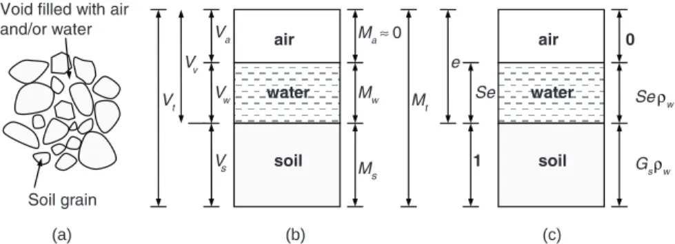
Here, Gs is the specific gravity of the soil grains, which is generally in the range 2.6-2.8. Dry density (d) is the density assuming the soil is dry and is Ms兾Vt.
Soil Classification
- Coarse-Grained Soils: Grain Size Distribution
- Fine-Grained Soils: Atterberg Limits
- Unified Soil Classification System
- Visual Identification and Description of Soils
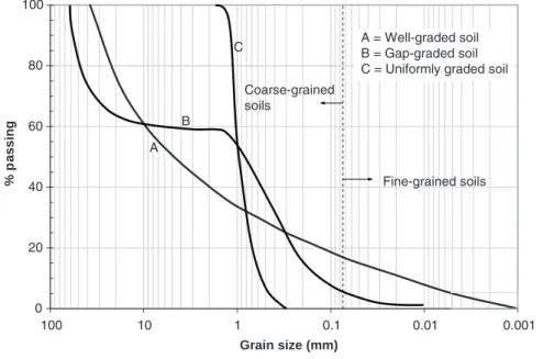
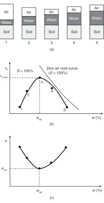
Fine-grained soil is classified as clay or silt according to Atterberg limits and not according to relative proportions. The fine-grained soil that occurs within the hatched area in Figure 1.5 is classified as CL-ML.
Compaction
- Compaction Curve and Zero Air Void Curve
- Laboratory Compaction Tests
- Field Compaction
The objective of these tests is to develop the compaction curve and determine the optimum water content and maximum dry density of a soil, with a specific compaction effort. The geotechnical properties of compacted clays are significantly affected by the water content of the leachate (Lambe 1958a, 1958b).
Flow through Soils
- Effective Stresses and Capillary
- Permeability
- Seepage
- Design of Granular Filters
The component carried by the soil framework is known as the effective stress or intergranular stress (σ′), and the water pressure in the voids is known as the neutral or pore water pressure (u). In impermeable rocks such as siltstones, the internal permeability can be on the order of 1 milli-Darcy.
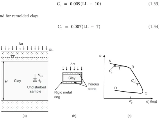
Consolidation
- Void Ratio vs. Effective Stress
- Rate of Consolidation
- Degree of Consolidation
The maximum hydraulic exit gradient (ieexit,max) that occurs along the dam wall can be estimated as 0.35. Terzaghi (1925) showed that the governing differential equation for the excess pore water pressure can be written as.
Shear Strength
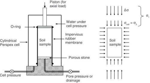
- Drained and Undrained Loading
- Triaxial Test
- Direct Shear Test
- Skempton’s Pore Pressure Parameters
- Stress Paths
The drawer can be drained or undrained depending on whether the drain valve is open or closed during this second phase. The effective stress parameters c′ and φ′ can be obtained from CD or CU tests, and the total stress parameters cu and φu are determined from UU tests.
Site Investigation
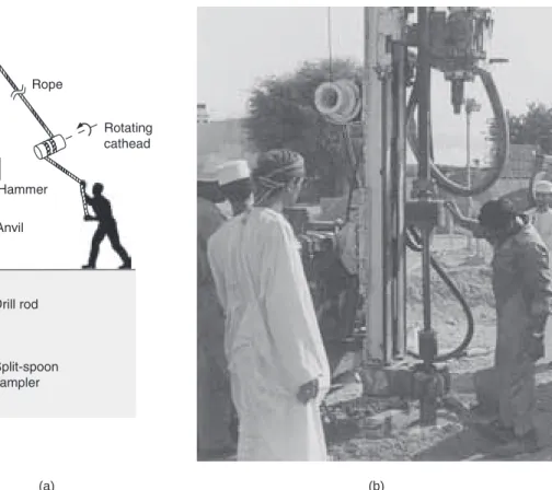
- Standard Penetration Test
- Static Cone Penetration Test and Piezocones
- Vane Shear Test
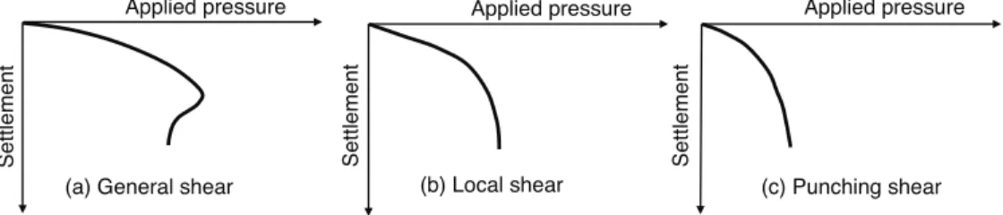
The actual energy delivered by the hammer to the split spoon sampler can be significantly less than the theoretical value, which is the product of the weight of the hammer and the fall. Using the pair of values for qc and fR, the soil type can be identified in Figure 1.24.
Soil Variability
With very limited geotechnical data derived from the laboratory and in situ tests for a project, it is not possible to obtain realistic estimates of the standard deviation of the soil parameters. Typical values of the coefficient of variation (COV) reported in the literature can be used as a basis for estimating the standard deviation of the soil parameters. 1983), and Baecher and Christian (2003) collected test data from various sources and presented the COV values.
Geotechnical Instrumentation
Settlement cells or slabs can be placed in dikes or foundations to monitor ongoing settlement. Horizontal inclinometers can be used to determine the settlement profile under a cross-section of a dike.
Introduction
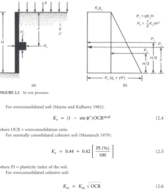
The magnitude of lateral earth pressure at any depth will depend on the type and amount of wall movement, soil shear strength, soil unit weight, and drainage conditions. The effective lateral earth pressure σ′h for this condition at any depth is called the resting earth pressure.
At-Rest Earth Pressure
The force per unit length of the supporting wall Po can be obtained by calculating the area of the pressure diagram, or The location of the line of action of the resultant can be obtained by taking the moment of the areas around the bottom of the wall or.
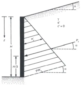
Rankine Active Pressure
Rankine Active Pressure with Inclined Backfill
The pressure σ′a will be inclined at an angle β with a plane drawn at right angles to the back side of the wall, and. The active force Pa per unit length of the wall can then be calculated as an angle. Determine the active force per unit length of the wall after the formation of a tensile crack and the location of the resulting Pa.
Coulomb’s Active Pressure
The active force Pa acts at a distance of H3 above the bottom of the wall and makes an angle δ′ with the normal drawn to the back of the wall.
Active Earth Pressure with Earthquake Forces
The active force Pae will incline at an angle δ′ with the normal drawn to the back of the wall. According to figure 2.9, Pa will act at a distance of H3 from the bottom of the wall. Note that Pae's line of action will be inclined at an angle of δ′ to the normal drawn to the back of the retaining wall.
Rankine Passive Pressure
The location of the working line z above the bottom of the wall can be obtained by taking the moment of the pressure diagram around the bottom of the wall, or .
Rankine Passive Pressure with Inclined Backfill
If the backfill of a frictionless retaining wall with a vertical back face (θ . = 0) is a c′-φ′ soil (see Figure 2.4), then the Rankine passive pressure at any depth z can be expressed as (Mazindrani and Ganjali 1997).
Coulomb’s Passive Pressure
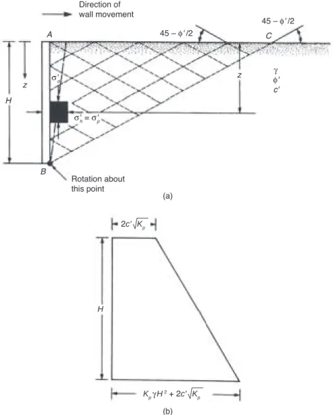
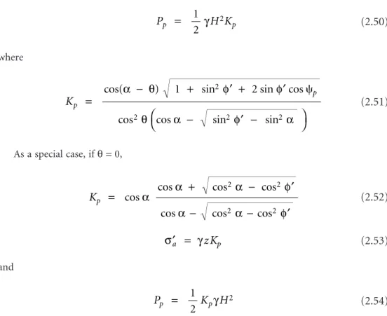
The Coulomb passive earth pressure per unit length of the wall can thus be given as It can be seen from this table that for a given value of φ′, the value of Kp increases with wall friction. Note that the resultant passive force Pp will act at a distance H3 from the bottom of the wall and will be inclined at an angle δ′ to the normal drawn to the back of the wall.
Passive Pressure with Curved Failure Surface (Granular Soil Backfill)
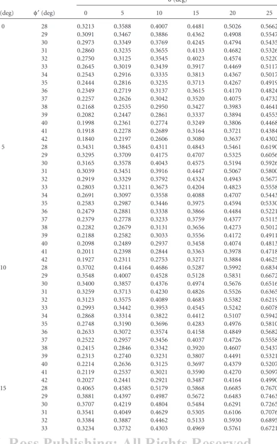
Several solutions have been proposed by different investigators to obtain the passive pressure coefficient Kp using a failure surface such as that shown in Figure 2.13. Shields and Tolunay (1973) used the disc method and obtained the variation of Kp for θ and α = 0. Zhu and Qian (2000) used the triangular disc method (such as in zone ABC in Figure 2.13) to obtain the variation of Kp .
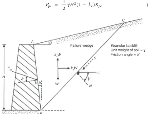
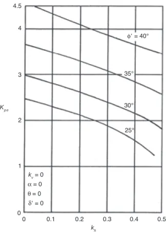
Passive Pressure under Earthquake Conditions (Granular Backfill)
The relationship for passive earth pressure in a retaining wall with a horizontal granular fill and vertical back face under earthquake conditions was evaluated by Subba Rao and Choudhury (2005) using the pseudo-static approach to the limit equilibrium method. Tables for the calculation of passive pressure, active pressure and bearing capacity of foundations, Gauthier-Villars, Paris. 6 Historical Developments • Terzaghi's bearing capacity equation • Meyerhof's bearing capacity equation • Hansen's bearing capacity equation • Vesic's bearing capacity equation • Gross and net pressures and bearing capacities • Pressure effects of water pre-pressure •.
Introduction
Stresses beneath Loaded Areas
- Point and Line Loads
兾 )
Uniform Rectangular Loads
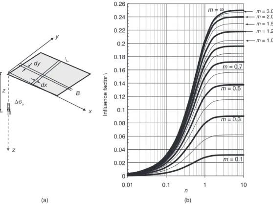
Boussinesq (1885) showed that in a homogeneous, isotropic elastic half-space, the vertical stress (∆σv) at a point in the medium increases due to a point load (Q) applied at the surface (see Figure 3.2). , is given by Using the equation or Figure 3.3b, the vertical stress increase at any point in the ground, under a uniformly loaded rectangular footing, can be found. Very often, the value of ∆σv is estimated by assuming that the applied earth pressure at footing level is distributed through a rectangular prism with slopes of 2 (vertical):1 (horizontal) in both directions, as shown in Figure 3.4.
Newmark’s Chart for Uniformly Loaded Irregular Areas
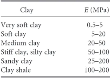
Bearing Capacity of Shallow Foundations
- Historical Developments
- Terzaghi’s Bearing Capacity Equation
- Meyerhof’s Bearing Capacity Equation
- Plane Strain Correction
- Eccentric Loading
- Hansen’s Bearing Capacity Equation
- Gross and Net Pressures and Bearing Capacities
- Effects of the Water Table
- Presumptive Bearing Pressures
Nc, Nq and Nγ are the bearing capacity factors, which are functions of the friction angle. Most theories of bearing capacity (eg, Prandtl, Terzaghi) assume that the base-soil interface is approx. If the water table extends to the base level, γm should be used in the second term and γ ′ in the third term in the bearing capacity equation.
Pressure Distribution beneath Eccentrically Loaded Footings
It can be seen from equation 3.71 that the soil pressure under the footing will be compressive at all points provided e < B兾6. Here the origin is at the center of the foot and the x and y axes are in the latitudinal and longitudinal directions respectively (see Figure 3.11b). Assuming the foundation load acts within this range, the contact stresses are compressive at all points below the footing.
Settlement of Shallow Foundations in Cohesive Soils
- Immediate Settlement
- Consolidation Settlement
- Secondary Compression Settlement
In a clay layer with an initial thickness of H and a void ratio of e0, the final consolidation setting sc due to the applied pressure q can be estimated from. The consolidation settlement s (t1) at a specific time t1 can be determined from the Uavg-T plot in Figure 1.17. Here, ep is the void ratio at the end of primary consolidation and Cα is the coefficient of secondary compression or the secondary compression index, which is determined from a consolidation test or can be estimated empirically.
Settlement of Shallow Foundations in Granular Soils
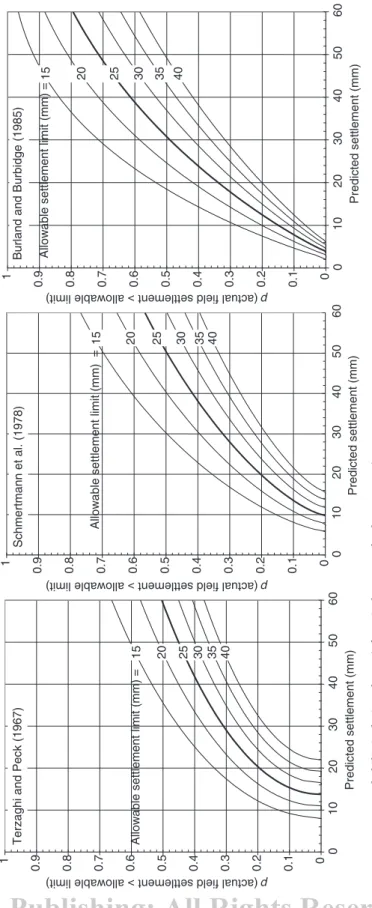
- Terzaghi and Peck Method
- Schmertmann et al. Method
- Burland and Burbidge Method
- Accuracy and Reliability of the Settlement Estimates and Allowable Pressures
- Probabilistic Approach
The allowable values of bearing capacity, based on the limiting settlement at 25 mm, estimated by the Burland and Burbidge (1985) and Terzaghi and Peck (1967) methods are shown in Figure 3.20. It can be seen in Figure 3.20 that the Burland and Burbidge (1985) method gives significantly smaller settlements and higher allowable pressures compared to the more conservative Terzaghi and Peck (1967) method. Three separate tables for the Terzaghi and Peck, Schmertmann et al., and Burland and Burbidge methods are given in Figure 3.21.
Raft Foundations
- Structural Design Methods for Rafts
- Bearing Capacity and Settlement of Rafts
The elastic constant of the soil is given by the subgrade reaction coefficient ks defined by equation 3.103. A major limitation of early flexible methods comes from unrealistic estimates of the subgrade reaction coefficient. The modulus of subgrade reaction can be obtained from a plate load test, typically using a 300 mm square plate.
Shallow Foundations under Tensile Loading
- Tensile Loads and Failure Modes
- Tensile Capacity Equations in Homogeneous Soils: Grenoble Model (Martin and Cochard 1973)
- Steeply Inclined Plates
In the shallow mode (Figure 3.27a.1 and b.1), the fracture surface reaches the ground plane, and all applied tensile loads are resisted by the plate. In the deep mode (Figure 3.27a.2 and b.3), the tensile load is shared by the slab and the shaft where the failure surface around the slab does not reach the ground level. The ultimate tensile load Qult obtained as a function of the plate depth in the shallow and deep modes is shown qualitatively in Figure 3.28.

Appendix A
Comparing examples 3 and 4, the smaller value Qult = 95.4 kN (slab at moderate slope) should be taken as the slab tensile capacity. Good engineering judgment is therefore required to select the strength parameters to be used in the design of sloped foundations in practice, due to the influence of the compacted backfill. D is the slab depth, pb is the slab perimeter, Sb is the slab surface, c is the soil cohesion, γ is the unit weight of the soil, W is the self-weight of the foundation element, and q0 is the external surcharge acting at ground level.
Appendix B
Introduction
In the case of foundation engineering, the system under consideration consists of three components: the structure, the structural foundation, and the supporting soil and rock media. The superstructure remains in firm contact with the structural foundation and the foundation is in contact with the supporting soil media. Forces transmitted from the superstructure to the foundation control the settlement of the foundation and supporting soil media.
Ross Publishing; All Rights Reserved 4-1
- Modeling of the Ground (Soil Mass) and Constitutive Equations
- Discrete Approach
- Continuum Approach
- Estimation of Model Parameters
- Modulus of Subgrade Reaction
- Elastic Constants
- Constants That Describe Two-Parameter Elastic Models of Soil Behavior
- Constants for Viscoelastic Half-Space Models The method of estimating the constants that describe the behavior of
- Application to Shallow Foundations
- Strip Footings
- Isolated Footings
- Combined Footings
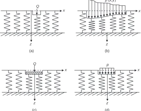
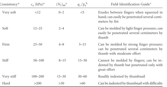
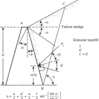
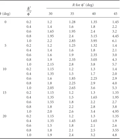
Due to the inherent complexity in soil mass behavior, various models have been developed to answer foundation-soil interaction problems. The surface displacements of the Winkler model are shown in Figure 4.1 for different types of loading. The value of the modulus of subgrade reaction was observed to depend on the depth of the soil layer.
The approach took into account the stress-strain-time response of the supporting soil medium (represented as a Kelvin model). Analysis of the soil-soil interaction problem was performed using the finite element method.