Glacial Ocean Dynamics: Insight from Deep-Sea Coral Reconstructions and A Time-Dependent Dynamical Box Model

(1)

Reconstructions and A Time-Dependent Dynamical Box Model

Thesis by

Sophia K.V. Hines

In Partial Fulfillment of the Requirements for the degree of

Doctor of Philosophy

CALIFORNIA INSTITUTE OF TECHNOLOGY Pasadena, California

2018

Defended September 5, 2017

(2)

ii

(3)

This thesis is dedicated to all the badass female scientists in my life.

(4)

iv

ACKNOWLEDGEMENTS

My graduate studies have been made possible with the love, support, and encour- agement of more people than can be named here, but I would like to take the time to acknowledge several who have been especially important.

First, my advisor Jess Adkins. You have pushed me to dig deeper, helped me see the bigger picture when I have gotten frustrated, and shaped me into the scientist that I am today. When you came to visit Carleton my senior year, I knew that I wanted to come to Caltech and work with you, and it is a decision that I have never regretted.

Andy Thompson, you have become a second advisor to me over the past year. Your endless patience and lack of judgment was always appreciated as I made my way from chemistry into the world of ocean physics.

I would like to thank John Eiler and Ken Farley, the other members of my committee.

You have helped me think critically about my data and your insight has greatly improved the work that I have done during my time at Caltech.

I had the great fortune of being able to spend time at the KCCAMS lab at UC Irvine.

I would like to acknowledge all of the members of the prep lab who have helped me over the years, and I would particularly like to thank John Southon for his generosity of time and lab space. Over the past few years I have also greatly enjoyed the chance to talk science with Patrick Rafter during my visits to UCI.

I always felt that I wouldn’t truly be an oceanographer until I got the chance to go to sea, and I am so happy that I got to do it with all the participants of IODP Expedition 361. Thanks to Ian, Sidney, Chad, and Leah for keeping everything running smoothly, and thanks to Andreas, Steve, Melissa, and Jason for keeping my spirits high 12 hours a day for two months.

I have been lucky enough to be a part of two lab groups during my time at Caltech, and I want to thank all the members (and affiliates) of the Adkins and Eiler lab groups. Nami, Guillaume, Stacy, Nithya, Katie, Uri, and Max were always there when I needed help in lab. Andrea, James, and Nithya were always game to talk with me about my data and your insights were always appreciated. I am grateful that I was able to go through grad school with my two classmates Adam and Ted—it won’t be the same without you guys.

I want to acknowledge the members of the pit, who helped me survive my first year,

(5)

and the members of Steuben House, who welcomed me when I first arrived. Life wouldn’t have been the same without all of my friends from the division. I have been grateful to share evening runs, early morning bike rides, trips to the climbing gym, and many backyard barbecues with all of you. Thanks to Jeff for sharing my love of bicycles, thanks to Hayden for matching my enthusiasm, and thanks to Nithya for helping me navigate academia as a woman and going on evening happy hour walks.

I want to say a very special ‘merci’ to Guillaume. You introduced me to lots of weird cinema and we shared many tasty Belgian beers. Your emotional and scientific support got me here today, and for that I will always be grateful.

Playing frisbee has been a huge part of my life in LA. My teammates have kept my mind and my body healthy through this process and I couldn’t imagine it any other way. I would particularly like to thank AJ, Joe, and Connie for helping me keep a good perspective on what is important in life.

I have been lucky enough to get to know Rob, Cyrus, Shannon, and Rachel through Adam and Hot Karate. Family weekends with all of you are always a blast and I hope there are more to come in the future.

I could not have done this without Adam. I am inspired by your creativity and intellect and you can always make me laugh. We have gone on some excellent adventures and cooked some tasty dinners. Plus you got me a dog.

Finally, my family. I owe my parents a million thank yous—your endless love and support has gotten me to where I am today. Thanks to Martha, Adriana, and Arielle for making my family bigger and filling my time at home with good food, tasty cocktails and lots of fun. Thanks to Peter and Barbara and the Miller-Midzik- Hallocks. You all count as family to me too.

(6)

vi

ABSTRACT

Glacial-interglacial cycles, occurring at a period of approximately 100,000 years, have dominated Earth’s climate over the past 800,000 years. These cycles involve major changes in land ice, global sea level, ocean circulation, and the carbon cycle.

While it is generally agreed that the ultimate driver of global climate is changes in insolation, glacial cycles do not look like insolation forcing. Notably, there is a highly non-linear warming response at 100,000 years to a relatively small forcing, implicating a more complicated system of biogeochemical and physical drivers. The ocean plays a pivotal role in glacial-interglacial climate through direct equator-to- pole transport of heat and its role in the carbon cycle. The deep ocean contains 60 times more carbon than the atmosphere, and therefore even small changes in ocean circulation can have a large impact on atmospheric CO₂, a crucial amplifier in the climate system. In order to better understand the role that ocean circulation plays in glacial-interglacial climate we focus on the last glacial-interglacial transition. In this thesis, we present reconstructions of changes in intermediate water circulation and explore a new time-dependent dynamical box model. We reconstruct circulation using radiocarbon and clumped isotope measurements on U/Th dated deep-sea corals from the New England and Corner Rise Seamounts in the western basin of the North Atlantic and from south of Tasmania in the Indo-Pacific sector of the Southern Ocean. Our new time-dependent model contains key aspects of ocean physics, including Southern Ocean Residual Mean theory, and allows us to explore dynamical mechanisms which drive abrupt climate transitions during the last glacial period.

In Chapter 2 we present a compilation of reconnaissance dated deep-sea corals from the Caltech collection. Reconnaissance dating facilitates sample selection for our high-precision radiocarbon and temperature time series and patterns in the depth distribution of deep-sea corals over time contain additional relevant climate information. In Chapter 3, we present a high-resolution radiocarbon record from south of Tasmania which highlights variability in Southern Ocean Intermediate Water radiocarbon during the deglaciation, particularly during the Antarctic Cold Reversal.

We use our radiocarbon data, in combination with other deglacial climate records, to infer changes in overturning circulation configuration across this time interval. In Chapter 4 we present our time-dependent dynamical box model. Our model displays hysteresis in basin stratification and Southern Ocean isopycnal outcrop position as

(7)

a function of North Atlantic Deep Water formation rate. In a dynamical system, hysteresis implies that there are multiple stable states, and switches between these states can lead to abrupt transitions, such as those observed during the middle of the last glacial period. In Chapter 5 we present paired radiocarbon and temperature time series from the North Atlantic and Southern Ocean spanning the late part of the last glacial. We explore the mechanisms driving trends in radiocarbon and temperature by looking at cross-plots of the data, and we make inferences about changes in circulation configuration using insight gained from our dynamical box model.

(8)

viii

PUBLISHED CONTENT AND CONTRIBUTIONS

Hines, Sophia K.V., John R. Southon, and Jess F. Adkins (2015). “A high-resolution record of Southern Ocean intermediate water radiocarbon over the past 30,000 years”. In:Earth and Planetary Science Letters 432, pp. 46–58. doi:10.1016/

j.epsl.2015.09.038.

S.K.V.H. helped to design this research, made all of the U/Th and radiocarbon measurements, analyzed the data, worked with J.F.A. to interpret the data, and wrote the manuscript with input from J.F.A. and J.R.S.

Contents reprinted with permission of Elsevier, the copyright holder.

Bush, Shari L. et al. (2013). “Simple, rapid, and cost effective: a screening method for¹⁴C analysis of small carbonate samples”. In:Radiocarbon55, pp. 631–640.

doi:10.1017/S0033822200057787.

S.K.V.H. helped prepare samples for radiocarbon analysis and provided some input on the manuscript.

Hines, Sophia K., John M. Eiler, and Jess F. Adkins (in prep.). “Deep-sea coral clumped isotope and radiocarbon records from North Atlantic and Southern Ocean intermediate water spanning the most recent glacial termination”. In:

S.K.V.H. helped to design this research, made all of the U/Th, radiocarbon, and clumped isotope temperature measurements, analyzed the data, worked with J.F.A. to interpret the data, and wrote the manuscript with input from J.F.A. and J.M.E.

Hines, Sophia K., Andrew F. Thompson, and Jess F. Adkins (in prep.). “Abrupt transitions and hysteresis in glacial ocean circulation explained by a two-basin time-dependent dynamical box model”. In:

S.K.V.H. helped to design this research, worked with A.F.T. to write the time- dependent box model, ran model experiments, worked with J.F.A. and A.F.T. to interpret the data, and wrote the manuscript with input from J.F.A. and A.F.T.

Thompson, Andrew F., Sophia K. Hines, and Jess F. Adkins (submitted). “A South- ern Ocean mechanism for climate transients through the last glacial period”. In:

Nature.

S.K.V.H. helped to design this research, worked with A.F.T. to write the time- dependent box model, contributed to the data interpretation, and helped write the manuscript.

(9)

LIST OF ILLUSTRATIONS

Number Page

2.1 Age-depth plot for Southern Ocean (A) and North Atlantic (B) corals.

Diamonds are data from Thiagarajan, Gerlach, et al. (2013) and squares are from this study. Lightest colored symbols (legend far right) are calculated using the IntCal13 calibration curve, medium colored symbols (legend center) are calculated using the Marine13 calibration curve, and darkest symbols (legend far left) are calculated using the Marine13 calibration curve and an additional reservoir correction of 400 years. . . 15 2.2 Comparison of Southern Ocean radiocarbon reconnaissance dates

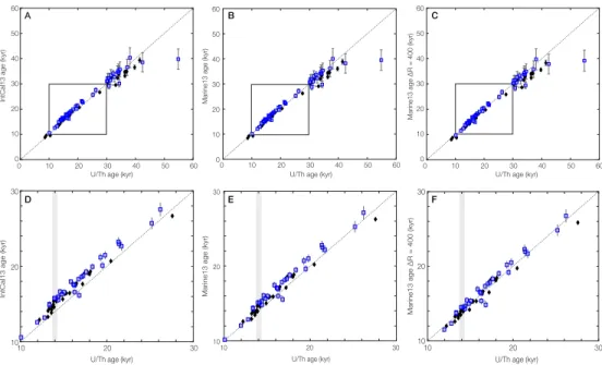
and precise U/Th ages. A) U/Th ages versus IntCal13-derived calendar ages, B) U/Th ages versus Marine13-derived calendar ages, and C) U/Th ages versus Marine13-derived ages with an additional reservoir age correction of 400 yr. D, E, and F are enlargements of boxed regions in A, B, and C, respectively. In all panels blue squares are dates from this study following the method of Bush et al.

(2013) and black filled diamonds are dates from Thiagarajan, Ger- lach, et al. (2013) following the method of Burke, Laura F. Robinson, et al. (2010). U/Th ages are reported in Chapter 3. Gray bars mark inflection in U/Th-age¹⁴C-age relationship at∼14 ka. . . 17 2.3 Comparison of North Atlantic radiocarbon reconnaissance dates and

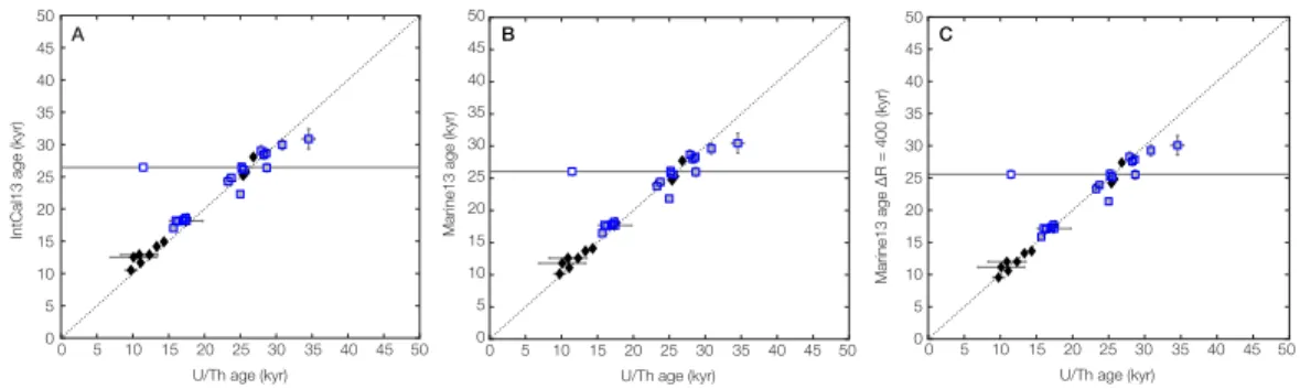
precise U/Th ages. A) U/Th ages versus IntCal13-derived calendar ages, B) U/Th ages versus Marine13-derived calendar ages, and C) U/Th ages versus Marine13-derived ages with an additional reservoir age correction of 400 yr. In both panels blue squares are dates from this study following the method of Bush et al. (2013) and black filled diamonds are dates from Thiagarajan, Gerlach, et al. (2013) following the method of Burke, Laura F. Robinson, et al. (2010). One sample (blue unfilled square) fell off the 1:1 line but has extremely large error bars (±95,000 yr on an age of 11,500 yr) due to high²³²Th (470,000 ppt). U/Th ages are reported in Chapter 5. . . 18

(11)

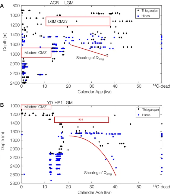
2.4 Annotated age-depth plot for Southern Ocean (A) and North Atlantic (B). Ages for all samples have been determined using the Marine13 radiocarbon calibration curve (Reimer, Bard, et al., 2013) with an additional reservoir correction of 400 years. Diamonds are from Thiagarajan, Gerlach, et al. (2013) and squares are from this study.

Boxes marking the locations of the modern OMZs are based on hydrographic data (Thiagarajan, Gerlach, et al., 2013). . . 19 3.1 Hydrography for the broader region around our sample location. A)

Sections of bomb-corrected∆¹⁴C (top), salinity (middle), and oxygen (bottom) from ~65°S to 10°S for the region marked on the inset map (Key et al., 2004). Sample location marked with a yellow star. Thick black contour lines are isopycnals (σ₁). In this region, tracers largely move along density surfaces. Map to the right shows the location of the sections, the Tasmanian coral location (yellow star) and the location of core MD-03-2611 (black star). B) Surface map of bomb- corrected ∆¹⁴C for the whole Southern Ocean. Thick black lines mark the positions of the major Southern Ocean fronts (from furthest north to furthest south: Subtropical Front (STF), Subantarctic Front (SAF), Polar Front (PF), Southern ACC Front (SACCF), and the Southern Boundary (SB)). C) Schematic Southern Ocean section with contours of density (taken from panel A). Coral location is marked with yellow star, and arrows show the two main ways to change radiocarbon values. D) Schematic of modern and glacial meridional overturning circulation with coral location marked with yellow star (adapted from (Ferrari et al., 2014)). In the modern, upper and lower cells are intertwined whereas in the glacial, cells are separated. This is due to increased sea ice extent (note: `₁ in the upper panel is greater than`₂in the lower panel). . . 51 3.2 Age-depth distribution for ¹⁴C screened corals. Upper panel shows

all screened corals (blue open circles;n = 508) and individuals that were selected for U/Th dating (blue filled circles; n = 112). Lower panel is an expanded view of the boxed region in the upper panel. In the lower panel, ¹⁴C screened and U/Th dated corals from the upper panel are shown in lighter blue, and filled blue circles represent the subset of U/Th dated samples that were also high-precision¹⁴C dated (n= 44). . . 56

(12)

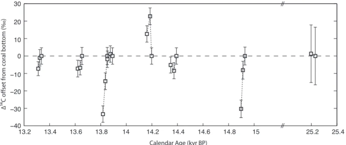
xii 3.3 Changes in∆¹⁴C over the lifetime of single deep-sea coral specimens.

Seven corals were sub-sampled for top–middle–bottom¹⁴C dates and one for top–bottom ¹⁴C dates. Calculated ∆¹⁴C values are plotted as differences from the bottom of the coral with 1σerror bars based only on uncertainty from radiocarbon dating. Of these eight corals, three show distinguishable changes in ∆¹⁴C over the lifetime of the coral, two show no change, and three show slight changes that are not resolvable within error. (Note break in x-axis between 15 and 25.2 ka.) 57 3.4 A) Tasmanian ∆¹⁴C record plotted with IntCal13 atmospheric∆¹⁴C

record, and B) converted into epsilon values. Error ellipses represent 1σ correlated U/Th and ∆¹⁴C errors. For epsilon values, these ellipses also take into account uncertainty in the IntCal13 atmospheric

∆¹⁴C record. Despite coming from between 1442 and 1947 m, epsilon variability between ~15–13 ka is not depth dependent. The deepest samples (at 1947 and 1898 m) are shown in panel B with dark gray filled circles, and they encompass nearly the full range in epsilon (including the highest point). The shallowest samples (at 1442 and 1599 m) are shown with white circles. 25 of the 30 samples from this time interval come from a depth range of less than 100 m (1599–1680 m). . . 58

(13)

3.5 ∆¹⁴C changes and frontal movement in the Southern Ocean. A) Atmospheric CO₂ curves from EPICA Dome C (through 22 ka) on the timescale of Lemieux-Dudon and Taylor Dome (20–25 ka) (In- dermühle et al., 2000; Lemieux-Dudon et al., 2010; Monnin et al., 2001) (light blue dots) and WAIS (Marcott et al., 2014) (dark blue circles and line) B) The IntCal13 atmospheric ∆¹⁴C reconstruction corrected for changes in atmospheric ¹⁴C production (Hain, Sig- man, and Haug, 2014). Arrow at top marks the initiation of CO₂ rise at ~18 ka. C) The Tasmanian coral ∆¹⁴C record, converted into epsilon. D-F) Foraminiferal species assemblages from core MD03-2611 (36°43.8'S, 136°32.9'E; 2420 m) located south of Aus- tralia (De Deckker et al., 2012). D) Percent abundance of subpolar foraminiferal species assemblage (N. pachyderma sinestral and T.

quinqueloba), indicative of SAF/PF movement. E) N. pacyderma dextral percent abundance, indicative of STF movement. F) G. ru- berpercent abundance, representative of the strength of the Lewellen Current. Black triangles at the bottom of the figure are age control points for MD03-2611 based on calibrated∆¹⁴C ages. . . 61

(14)

xiv 3.6 Opal flux and epsilon radiocarbon records from the Southern Ocean

across the deglaciation. A) Opal flux record from Indo-Pacific core E27-23 (59.62°S 155.24°E, 3182 m). B) Opal flux record from South Atlantic core TN057-13 (53.1728°S 5.1275°E, 2848 m). Error bars on opal flux values are the size of the points. Also included are chronological constraints (from calibrated¹⁴C dates) for both cores, with E27-23 tie points in filled black triangles and TN057-13 tie points in open blue triangles. C) Tasmanian coral∆¹⁴C record shown as epsilon units offset from the atmosphere with other Southern Ocean records ∆¹⁴C records. Deep South Atlantic (L. C. Skinner et al., 2010) (brown ellipses and upward-facing triangles; core MD07-3076;

44.1°S 14.2°E, 4981 m), southern Drake Passage UCDW (Burke and L F Robinson, 2012) (dark blue ellipses and right-facing triangles;

~60°S, ~1000 m), northern Drake passage AAIW (Burke and L F Robinson, 2012) (dark teal ellipses and left-facing triangles; ~55°S, 500 m), Chilean Margin (De Pol-Holz et al., 2010) (teal ellipses and diamonds; core SO161-SL22; 36.2°S 73.7°W, 1000 m), Chatham Rise (L. Skinner et al., 2015) (purple ellipses and upward-facing triangles; core MD97-2121; 40.4°S 178.0°E, 2314 m), and Tasma- nia (this study) (red ellipses and circles; ~45°S, ~1600 m). “T, M, B” labels refer to top, middle, and bottom ¹⁴C values for individual corals. Of corals with top, middle, and bottom dates, only three show resolvable changes over the coral’s lifespan (see Figure 3.3). The direction of these changes is marked with an arrow. Top right: map showing the locations of cores TN057-13 and E27-23, Drake Pas- sage Corals and Tasmanian corals. Bottom left: schematic showing modern Southern Ocean zonally-averaged isopycnal structure, Drake Passage location, and locations of epsilon records (in color-coded symbols). . . 63

(15)

3.7 Records of the full deglacial period showing changes in overturning circulation. A) NGRIPδ¹⁸O from Greenland (Andersen et al., 2006;

Rasmussen et al., 2006). B) Hulu cave δ¹⁸O from stalagmites H82 (blue) and YT (green) (Wang et al., 2001). C) WAIS Divide δ¹⁸O from west Antarctica (WAIS Divide Project Members, 2013). D) Atmospheric CO₂ from WAIS Divide (Marcott et al., 2014). E)

∆¹⁴C record from south of Tasmania represented as epsilon (this study). F) Tasmanian∆¹⁴C record with other Southern Ocean∆¹⁴C records (same colors and symbols as Figure 3.6C) (Burke and L F Robinson, 2012; De Pol-Holz et al., 2010; L. C. Skinner et al., 2010;

L. Skinner et al., 2015). . . 67 3.8 Error on ∆¹⁴C as a function of coral age, calendar age error, and

radiocarbon age error. Error on ∆¹⁴C is calculated as a function of relative calendar age error for corals of three different ages. The dashed line is for a Fm of ±0.0002 based on calcite blanks and the solid line is for a Fm error of ±0.0007 based on measured deep-sea corals. . . 76 3.9 Benthic-Planktic age offsets for Southern Ocean foram records. Data

from De Pol-Holz (De Pol-Holz et al., 2010) (light blue diamonds, core SO161-SL22; 36.2°S 73.7°W, 1000m), Skinner (L. Skinner et al., 2015) (light green inverted triangles, core MD97-2121; 40.4°S 178.0°E, 2314m) and (L. C. Skinner et al., 2010)(dark blue triangles, core MD07-3076; 44.1°S 7.8°E, 4981m), and Rose (Rose et al., 2010) (green circles with black vertical lines connecting B-P ages calculated using different planktic foram species from the same core depth, core MD97-2120; 43.5°S 174.9°E, 1210 m). Rose et al. B-P data plotted using aδ¹⁸O-based age model that is independent of¹⁴C (from their Table S2). These results cover a limited period from 18 to 16 ka and the planktic data show interspecies age differences of up to 1800

14C-years. . . 77 3.10 ∆¹⁴C records from south of Tasmania and the Brazil Margin (Mangini

et al., 2010). Black curve is IntCal13, red ellipses are Tasmanian coral

∆¹⁴C data, and blue ellipses are Brazil Margin ∆¹⁴C data. Ellipses drawn with 1σU/Th and¹⁴C errors. . . 78

(16)

xvi 4.1 Greenland and Antarcticδ¹⁸O records with Pa/Th circulation tracer.

Oxygen isotopic composition of NGRIP ice core in Greenland (A) and EDML ice core in Antarctica (C). The δ¹⁸O composition of ice is a proxy for regional temperature. Numbers mark the Dansgaard- Oeschger (DO) events in Greenland and corresponding AIM events in Antarctica. B) Compilation of Pa/Th records from the Bermuda Rise (youngest section from McManus et al. (2004) (diamonds), middle section from Lippold et al. (2009) (circles), oldest section from Böhm et al. (2015) (squares)). Pa/Th ratio is a proxy for the strength of North Atlantic Deep Water (NADW). Horizontal dashed line marks the Pa/Th production ratio of 0.093. Bar at top shows the Marine Isotope Stage boundaries. . . 87 4.2 Schematic of model architecture. Model domain is split into an

Atlantic sector and an Indo-Pacific sector. Each basin has a channel region with sloping isopycnals that outcrop at the surface (from -` to 0), and a basin region where isopycnals are flat-lying (from 0 to Lb). Within each basin, water can move between density classes due to diabatic processes at the surface of the channel region or due to diapycnal diffusion in the basin region. Water can move between the Atlantic and Indo-Pacific due to zonal convergence in the channel (pink arrows) or via the Indonesian Throughflow (blue arrow). At the northern end of the Atlantic basin, North Atlantic Deep Water is formed with variable density (green arrow; density specified by parameter φ). Two plots in upper left show wind stress, τ, (top) and surface buoyancy flux, Fb, (bottom) as a function of y for the channel region of the model. Model solves for the outcrop positions of isopycnals in the channel, y, and depths of isopycnals in the basin,z. 92 4.3 Example of model response in transient experiment. Top panel shows

NADW forcing, middle panel shows outcrop position (as fraction of total ACC width), and bottom panel shows interface depth in the basin. Legend shows colors for the three interfaces and shading in middle panel indicates regions of positive and negative buoyancy forcing at the surface of the Southern Ocean,Fbplotted to right. This experiment was run at φ = 1, meaning all of the NADW flux went from layer 1 into layer 3. . . 98

(17)

4.4 Outcrop position of interface 2 in the Atlantic (y^A

2) for all values of φ. φvaries from 0 to 1 in increments of 0.1. Each loop is a different single color; dashed lines mark the up-going limb of the loop (i.e.

increasing from 4 Sv to 20 Sv) and solid lines mark the down-going limb of the loop. Circles mark each NADW flux value that was run.

Shading in the background indicates regions of positive and negative surface buoyancy flux, Fb (plotted in full to right). Horizontal line marks the Fb=0 contour. . . 100 4.5 Equilibration time for interfacey^A

2 for all values ofφas a function of NADW flux. Filled circles are for the up-going limb of the loop and unfilled circles are for the down-going limb. Color and size of circle corresponds to equilibration time. . . 101 4.6 Outcrop position of y^A

2 as a function of NADW flux for different sea ice extents (ysi). A ysi value of -0.5 means that the maximum ofFb

associated with sea ice melt is centered at the middle of the ACC and is an equivalent position to -0.5 on the y axis (see Equation 4.7).

From bottom to top, ysi position increases in increments of 0.05.

φ=1 for all experiments. . . 102 4.7 Interface 2A slope as a function of NADW flux forφ=1. The slope

for interface 2 in the Atlantic is defined as−z^A

2/y^A

2. Horizontal line markss =s₀. . . 103 4.8 Perturbation experiments to test the stability of the hysteresis loop.

Starting with the steady-state interface positions for a NADW flux of 8.75 Sv on the upper limb of the hysteresis loop, z^A

2 and z^P

2 were displaced and then allowed to relax for 50, 200, and 500 years (y^A

2

for each of these simulations are plotted in circles, diamonds and squares, respectively). . . 104 4.9 Perturbation experiments in z space. Same experiment as shown in

Figure 4.8. Vertical diffusivity profile is also shown with diffusivity transition depth (1600 m) and diffusivity transition width (d = 300 m) marked. . . 105

(18)

xviii 4.10 Outcrop position of y^A

2 as a function of NADW flux for different vertical diffusivity profiles. The control experiment has a kinked κ profile (green). A series of experiments with constant κ(at values of 0.2×10⁻⁴, 0.6×10⁻⁴, and 1×10⁻⁴; red) and an experiment with a linearly increasing κprofile (from 0.2×10⁻⁴to 1×10⁻⁴; black) are shown for comparison. . . 106 4.11 Assessment of circulation configuration for allφexperiments. Com-

binations of NADW strength and density that have very little zonal transport in layers 3 and 4 lead to a circulation configuration that is two-cell-like and combinations of NADW strength and density that have large zonal transport in layers 3 and 4 lead to a circulation configuration that is more figure-eight-like. Different colored circles represent different φ values from 0 (at top) to 1 (diagonal to lower right corner). Shaded regions show location of the modern ocean and approximate locations for the LGM and MIS 3. The high density of circles in the MIS 3 region mark the hysteresis loops, which show separation in outcrop position but not in circulation configuration. . . 107 4.12 Assessment of circulation configuration for all ysiexperiments. The

relationship between NADW flux and circulation configuration is quite similar between all of the ysi experiments compared to the φ experiments (see Figure 4.11). The experiment with ysi = −0.5 is (labeled) is the same as theφ= 1 experiment in Figure 4.11. . . 110 5.1 Modern hydrography from the Southern Ocean. A) Surface plots

of temperature and ∆¹⁴C (NAT14C variable from the GLODAP database) (Key et al., 2004). B) Cross-plot of modern potential temperature and ∆¹⁴C data from section highlighted on map (lower right). Data are segregated by depth and latitude. Sample location is marked with a star. . . 121 5.2 Modern hydrography from the North Atlantic. Sections of ∆¹⁴C

(NAT14C variable from the GLODAP database) (A) and potential temperature with overlaid salinity contours (B) (Key et al., 2004).

Section highlighted on map. C) Cross-plot of data from sections segregated by latitude with water masses highlighted. On sections, the triangle marks location of Corner Rise Seamounts and the square marks location of New England Seamounts. . . 122

(19)

5.3 Summary of carbonate standard data. A) Plot of standard residuals in the absolute reference frame on an arbitrary time axis, where the standard residual is defined as: measured∆₄₇−accepted∆₄₇. B) Same data as in A, but now grouped by measurement week. C) ∆₄₇ data for deep-sea coral standard LB-001 versus time, with measurement intervals labeled. Solid horizontal line is the long-term average ∆₄₇ value for LB-001, 0.850, and dashed horizontal line is the accepted

∆₄₇from the coral growth temperature. Blue points were measured on the instrument ‘Admiral Akbar’ and red points were measured on the instrument ‘Princess Leia’. Colored bars at the top of the plot indicate four separate aliquots of the coral that were cut and measured—long- term variation in measured ∆₄₇ does not correspond to times when new aliquots were taken. . . 127 5.4 Transferring deep-sea corals run by N. Thiagarajan into the ARF. Sec-

ondary transfer function and deep-sea coral temperatures converted into the absolute reference frame. . . 129 5.5 Clumped isotope temperature records for the North Atlantic and

Southern Ocean. In order to better visualize long-term trends in the data, North Atlantic and Southern Ocean records were interpolated at 10-year resolution and smoothed using a 500-year Gaussian filter. Error envelope is average 1SE temperature error for North Atlantic and Southern Ocean (1.3 and 1.1^◦C respectively). . . 130 5.6 ∆¹⁴C records from the North Atlantic and Southern Ocean. Coral

∆¹⁴C values are plotted with 1σ error ellipses that take into account correlated U/Th age and¹⁴C date error. IntCal13 atmospheric∆¹⁴C record is also plotted for reference (Reimer, Bard, et al., 2013). . . 132 5.7 Deep-sea coral radiocarbon and temperature records from the North

Atlantic (yellow) and Southern Ocean (blue). ∆¹⁴C converted into ¹⁴C using the IntCal13 atmospheric radiocarbon curve (Reimer, Bard, et al., 2013). Temperature converted into potential temperature using each coral’s collection depth and latitude. . . 133

(20)

xx 5.8 Cross-plots of Southern Ocean (A) and North Atlantic (B) radiocar-

bon and temperature data. Radiocarbon data are converted into¹⁴C and temperatures are converted into potential temperature. Time peri- ods are: ‘pre-LGM’ (>22 ka), ‘LGM’ (17.5–22 ka), ‘HS1’ (15.1–17.6 ka), and ‘ACR’ (<15.1 ka). Modern potential temperature and radiocarbon (‘NAT14C’) data from the GLODAP database are plotted in the background (Key et al., 2004). Modern value is marked with a black star. . . 133 5.9 Compiled climate records spanning the late glacial. From top: High-

latitude insolation curves (Huybers and Eisenman, 2006), North GRIPδ¹⁸O on the GICC05 chronology (Rasmussen et al., 2014; An- dersen et al., 2004), WAISδ¹⁸O on the WD2014 chronology (WAIS Divide Project Members, 2013; Buizert et al., 2015), atmospheric pCO₂ from WAIS (open circles and line) (Marcott, Bauska, et al., 2014), EDC (circles) (Monnin et al., 2001; Lemieux-Dudon et al., 2010), and Taylor Dome (filled circles) (Indermühle et al., 2000), Pa/Th from the Bermuda rise (purple diamonds) (McManus et al., 2004) and ODP 1063 (blue squares) (Lippold et al., 2009), Hulu cave δ¹⁸O from stalagmites PD (orange) and MSD (yellow) (Y. J.

Wang et al., 2001), atmospheric∆¹⁴C from IntCal13 (Reimer, Bard, et al., 2013), and the atmospheric∆¹⁴C record corrected for production (Hain, Sigman, and Haug, 2014). Light grey bars mark times of decreased NADW flux according to Pa/Th, dark grey bars mark weak monsoon intervals, and dates of Heinrich events are marked by triangles at the top of the figure (Hemming, 2004). . . 134 5.10 Contour plots of temperature (top) and radiocarbon (bottom) from the

western North Atlantic. Compiled temperature records are based on deep-sea coral clumped isotope measurements (Thiagarajan, Subhas, et al., 2014, and this study) and benthic foram (Marcott, Clark, et al., 2011) and ostracode (Dwyer et al., 2000) Mg/Ca measurements.

Deep-sea coral (Eltgroth et al., 2006; Laura F. Robinson et al., 2005;

Adkins, Cheng, et al., 1998; Thiagarajan, Subhas, et al., 2014, and this study) and benthic foram (Laura F. Robinson et al., 2005; Keigwin and Schlegel, 2002; Keigwin, 2004)∆¹⁴C values were converted into ¹⁴C using the IntCal13 atmospheric radiocarbon curve (Reimer, Bard, et al., 2013). . . 135

(21)

5.11 Schematic of circulation changes across the late glacial. North and south deep-sea coral approximate sample locations marked with stars. 139 5.12 Contour plots of temperature (top) and radiocarbon (bottom) from

the Southern Ocean. Temperature records based on Mg/Ca measurements on benthic foraminifera (Roberts et al., 2016) and clumped isotope measurements on deep-sea corals (this study). Radiocarbon measurements from benthic foraminifera (De Pol-Holz et al., 2010;

L. Skinner et al., 2015; L. C. Skinner et al., 2010; Barker, Knorr, et al., 2010) and deep-sea corals (Hines, Southon, and Adkins, 2015).

∆¹⁴C values were converted into¹⁴C using the IntCal13 atmospheric radiocarbon curve (Reimer, Bard, et al., 2013). . . 140 5.13 Correlation between ¹⁴C and potential temperature. A) ¹⁴C and

potential temperature records with interpolated data. Arrows show the direction of change for top-bottom radiocarbon and temperature data. B) Cross plots of interpolated ¹⁴C and potential temperature with black line connecting actual measured data points. Colorbar shows age in kiloyears. . . 143 5.14 Deep-sea coral intermediate water radiocarbon data from the ACR.

A) Time series of¹⁴C from south of Tasmania and the Drake Passage (Burke and L F Robinson, 2012; Chen et al., 2015). B) Latitude- depth contour plot of¹⁴C from 14.2–13.1 ka (boxed interval in panel A). Locations of deep-sea coral data marked with open symbols and approximate Drake Passage latitude marked at top. . . 144 5.15 Modern salinity section from south of Tasmania with contours of

dissolved oxygen. Labels mark the relative position of water masses in the area south of Tasmania. Deep-sea corals sit at∼44.5^◦S, 1600 m, near the boundary between AAIW and PDW. . . 153

(22)

xxii

LIST OF TABLES

Number Page

2.1 Southern Ocean reconnaissance dates. Samples marked with reference “NT” were screened according to the method of Burke, Laura F.

Robinson, et al. (2010) by Thiagarajan, Gerlach, et al. (2013). Sam- ples with reference “SH” were screened for this study according to the method of Bush et al. (2013). Radiocarbon-dead samples are assigned a dummy value of 60,000 with no error on the age. . . 23 2.2 North Atlantic reconnaissance dates. Samples marked with refer-

ence “NT” were screened according to the method of Burke, Laura F.

Robinson, et al. (2010) by Thiagarajan, Gerlach, et al. (2013). Sam- ples with reference “SH” were screened for this study according to the method of Bush et al. (2013). Radiocarbon-dead samples are assigned a dummy value of 60,000 with no error on the age. . . 36 3.1 Summary of U/Th dates including measured uranium and thorium

concentration and uranium isotope ratios. Corrected age takes into account initial thorium using an atom ratio of²³⁰Th/²³²Th = 80±80.

δ²³⁴Ui is initialδ²³⁴U corrected using measured age. Both raw and corrected ages are in yr since 1980. ∗samples flagged for high²³²Th (>2000 ppt). †samples flagged for non-marineδ²³⁴Ui(where marine is defined as 147±7 for samples younger than 17 ka and 141.7±7.8 for samples older than 17 ka by IntCal09). ‡samples are flagged for both criteria. . . 79 3.2 Summary of radiocarbon dates used for calculating∆¹⁴C. . . 83 4.1 Values and definitions of parameters used in model. . . 93 5.1 Summary of Southern Ocean and North Atlantic clumped isotope

temperature data. All reported ∆₄₇ values and temperatures have been corrected with deep-sea coral standard LB-001. . . 154

(23)

5.2 Summary of North Atlantic U/Th dates including measured uranium and thorium concentration and uranium isotope ratios. Corrected age takes into account initial thorium using an atom ratio of²³⁰Th/²³²Th

= 80±80. δ²³⁴Uiis initialδ²³⁴U corrected using measured age. Both raw and corrected ages are in yr since 1980. ∗ samples flagged for high ²³²Th (>2000 ppt). † samples flagged for non-marine δ²³⁴Ui

(where marine is defined as 147±7 for samples younger than 17 ka and 141.7±7.8 for samples older than 17 ka by IntCal09). ‡samples are flagged for both criteria. . . 156 5.3 Summary of radiocarbon dates used for calculating∆¹⁴C.∗samples

flagged for high²³²Th (>2000 ppt). †samples flagged for non-marine δ²³⁴Ui(where marine is defined as 147±7 for samples younger than 17 ka and 141.7±7.8 for samples older than 17 ka by IntCal09). ‡ samples are flagged for both criteria. . . 158

(24)

1 C h a p t e r 1

INTRODUCTION

For nearly a million years, the earth’s climate has been typified by glacial-interglacial cycles, occurring at a period of roughly 100,000 years (Lisiecki and Raymo, 2005).

These glacial cycles were accompanied by changes in global temperature, atmospheric CO₂, land-based ice sheets, and global sea level (Jouzel et al., 2007; Lüthi et al., 2008; Rohling et al., 2014). While the ultimate driver of these cycles is generally accepted to be changes in high-latitude insolation, or solar radiation, the character of these late-Pleistocene glaciations does not match the shape of insolation curves (Milanković, 1941; Hays, John Imbrie, and Shackleton, 1976; J Imbrie, Boyle, et al., 1992; J Imbrie, Berger, et al., 1993). In particular, glacial cycles are characterized by an abrupt non-linear response at roughly 100,000 years, while high-latitude insolation has much higher spectral power at 20,000 and 40,000 years.

This has led to discussion of whether glacial cycles are paced by sets of 20-kyr procession cycles (Cheng, Edwards, et al., 2016), 40-kyr obliquity cycles (Huybers and Wunsch, 2005), or some combination of both (Huybers, 2011). Recently, some of the discussion has moved away from trying to quantify the exact sequence of events that led to each glacial termination and focused instead on how the build-up of potential energy in the climate system could lead to certain insolation maxima triggering interglacials while others do not (Tzedakis et al., 2017). This potential energy could take the form of deep ocean heat, stored CO₂, large land-based ice sheets, or some other aspect of the climate system that is able to respond in a non-linear way. The question now is: what combination of glaciological, biogeochemical, and physical ocean processes allowed for the necessary build-up of energy in the climate system, and what did that build-up of potential energy look like?

One crucial amplifier in the climate system is the carbon cycle. Although evidence suggests that atmospheric CO2 does not precede temperature rise at deglaciations (Caillon et al., 2003), CO₂concentrations have varied along with temperature over the past 800,000 years (Lüthi et al., 2008). Carbon dioxide is a greenhouse gas, and therefore compounds the effects of changes in insolation. Although atmospheric CO₂ has the largest direct effect on global temperature, it is one of the smallest reservoirs in the global carbon system (Sigman and Boyle, 2000). The deep ocean contains 60 times more carbon than the atmosphere, and therefore changes in ocean

(25)

circulation and biogeochemistry can have a large impact on atmospheric CO₂. One way that ocean biogeochemistry can impact atmospheric CO₂ is through the efficiency of the biological pump (Sigman, Hain, and Haug, 2010). The “biological pump” refers to the mechanism by which organisms in the surface ocean fix CO₂ into organic matter and the fixed organic carbon is exported into the deep ocean. In the modern ocean, deep water sinking in the North Atlantic has very low dissolved phosphate because organisms living in the surface water have consumed all of it in order to fix CO₂ into organic carbon. In the Southern Ocean, however, newly formed deep water still has unconsumed phosphate, which represents excess CO₂ left in the atmosphere. As was pointed out in the “Harvardton Bears” models, a 100% efficient biological pump cannot achieve the full interglacial-glacial CO₂ draw down—these simple box models require a combination of increased biological pump efficiency and circulation slow-down (Knox and McElroy, 1984; Siegenthaler and Wenk, 1984; Sarmiento and Toggweiler, 1984).

Ocean circulation impacts global climate in two main ways: it provides a means of sequestering CO₂from the atmosphere via the biological pump and it participates in direct equator-to-pole heat transport (Ganachaud and Wunsch, 2000; L. D. Talley, 2003). The meridional overturning circulation represents the ocean circulation path that transfers water from the surface to the deep and back, and it occurs on timescales of∼1000 years, allowing deeply regenerated CO2to be sequestered from the atmosphere for thousands of years (Stuiver, Quay, and Ostlund, 1983). There are two places where deep water is formed in the ocean: the North Atlantic (in the Labrador and Nordic Seas) and the Southern Ocean (on continental shelves in the Weddell Sea, Ross Sea, and around East Antarctica) (Kuhlbrodt et al., 2007).

The modern ocean has a “figure-eight” circulation, meaning that its closure involves separate but equally important processes in both the Atlantic and Indo-Pacific basins (Lumpkin and Speer, 2007; L. Talley, 2013). This figure-eight structure involves a central role for the Southern Ocean and is lost in zonally averaged depictions of the overturning circulation, which instead show two stacked counter-rotating cells.

In order to understand the details of the modern overturning circulation and how it may have changed in past climates it is crucial to understand the circulation of the Southern Ocean. The Southern Ocean is unique because it is the only place where there are no continental impediments to zonal flow. Strong westerly winds over the Southern Ocean lead to the generation of the Antarctic Circumpolar Current (ACC), which, at around 140 Sv (1 Sv is 10⁶ m³ s⁻¹), is the largest current in the

(26)

3 world. Because there are no continental boundaries in the Drake Passage latitude band above the depth of the Scotia Ridge, north-south flow cannot be generated via zonal pressure gradients, as is the case in the ocean basins. Modeling and obser- vational data from the Southern Ocean show an interesting density structure—deep isopycnals, or density surfaces, slope to the surface across the ACC, transforming the vertical density gradient, which characterizes the ocean basins, into a meridional density gradient at the surface (Doos and Webb, 1994; Speer, Rintoul, and Sloyan, 2000).

Over the past two decades a new theory has emerged to explain meridional overturning circulation in the Southern Ocean. This Residual Mean theory builds on observations of the Southern Ocean isopycnal structure, and is based on a balance between wind and eddies. Southern Ocean westerly winds drive northward Ekman transport and steepen isopycnals. Steep isopycnals become baroclinically unstable and generate eddies that act to relax isopycnal slopes (Marshall and Radko, 2003).

In the subsurface, flow occurs adiabatically along isopycnals. Overturning transport is achieved as a result of buoyancy fluxes at the surface which allow water to be transformed to heavier or lighter density classes according to the equation:

ψr es = ψ¯ +ψ^∗, or rewritten : (1.1) B₀

∂b₀/∂y = − τ

ρ₀f +K sρ (1.2)

where ¯ψ is the wind-driven mean component, ψ^∗ is the eddy-driven component, ψr es is the buoyancy-driven residual component, B₀ is the surface buoyancy flux,

∂b₀/∂yis the surface buoyancy gradient,τis the surface wind stress, ρ₀is the mean ocean density, f is the coriolis parameter, K is the eddy diffusivity, and sρ is the isopycnal slope. There are positive surface buoyancy fluxes in the northern part of the Southern Ocean due to a combination of direct heating by the atmosphere, precipitation minus evaporation, and freshwater from sea ice melt (Abernathey et al., 2016). There are negative surface buoyancy fluxes in the southern part of the Southern Ocean due to brine rejection and direct heat loss to the atmosphere within leads in the sea ice known as polynyas (Abernathey et al., 2016; Nicholls et al., 2009). There is a split in the circulation, therefore, with a clockwise overturning cell in regions of positive surface buoyancy forcing (sometimes called the upper cell) and a counter-clockwise overturning cell in regions of negative surface buoyancy forcing (the lower cell).

(27)

In the modern ocean, North Atlantic Deep Water (NADW) upwells in a region of the Southern Ocean where it experiences a negative surface buoyancy forcing, causing it to flow south and sink again as Antarctic Bottom Water (AABW) (L. Talley, 2013).

If this newly formed AABW flows back into the Atlantic, it diffusively upwells back into NADW. If, instead, it flows into the Indian or Pacific basins, it is able to diffusively upwell further in the water column to a lighter density class. Therefore, when this water returns to the Southern Ocean as Indian Deep Water or Pacific Deep Water (IDW/PDW), it upwells in a region of positive surface buoyancy forcing (L.

Talley, 2013). Finally, this water flows to the north again as Antarctic Intermediate Water (AAIW) and Subantarctic Mode Water (SAMW). These relatively shallow water masses can be transformed, via downward heat diffusion, to upper ocean subtropical waters, which eventually make their way to the North Atlantic, closing the overturning circulation (L. Talley, 2013; Lozier, 2010). This three-dimensional figure-eight structure is lost in some depictions of the overturning circulation where zonal averaging hides the separate but equally important processes that occur in the different ocean basins.

Since ocean circulation has such a strong impact on global climate, a natural question is: how did the structure and rate of ocean circulation change across glacial- interglacial cycles? There is paleoceanographic evidence that ocean circulation looked quite different during the Last Glacial Maximum (LGM, ∼22–18 ka) than it does today. A reconstruction of δ¹³C in the western Atlantic during the LGM shows a shoaled NADW and expanded AABW compared to the modern (Curry and Oppo, 2005). δ¹³C is a non-conservative circulation tracer, which can track the difference between northern and southern-source water in the Atlantic. Another study combined depth transects of δ¹³C and δ¹⁸O in the Atlantic at the LGM to construct a tracer transport budget and constrain the ratio of overturning transport to vertical mixing (Lund, Adkins, and Ferrari, 2011). They found that in addition to its shoaled configuration, there was also greater stratification between glacial NADW and AABW.

A theoretical scenario has been proposed to explain the change in circulation configuration at the LGM (Ferrari et al., 2014). Ferrari et al. (2014) point out that the switch between negative and positive buoyancy forcing in the Southern Ocean is aligned with the quasi-permanent sea ice edge, and this therefore marks the boundary between the upper and lower circulation cells. To first order, isopycnal slopes are constant across the ACC and therefore the depth of the boundary between the upper

(28)

5 and lower circulation cells can be calculated geometrically (Ferrari et al., 2014). In the modern ocean this depth comes out to around 2200 m, below the mean depth of rough topography on the seafloor (∼2000 m). Rough topography greatly increases diapycnal mixing in the deep ocean (Polzin et al., 1997), and the deep boundary between the circulation cells could therefore contribute to the modern figure-eight circulation structure (Ferrari et al., 2014). At the LGM, paleo data and models suggest that sea ice was expanded by at least 5^◦(Ferrari et al., 2014; Gersonde et al., 2005; Roche, Crosta, and Renssen, 2012). By the same geometric argument, this would shift the surface boundary between the upper and lower circulation cells to the north and shoal it in the basins by around 500 m (Ferrari et al., 2014). This could contribute to the shoaling of NADW and would potentially switch the circulation configuration into a “two-cell” state, with greater stratification and separation between the circulation cells (Ferrari et al., 2014). A switch to two-cell circulation at the LGM should appear in radiocarbon data as an age maximum at mid-depth (Burke et al., 2015), which is indeed what shows up in a recent compilation of LGM data by Skinner et al. (2017).

In this thesis, we investigate two questions: how did the structure of ocean circulation change during the late part of the last glacial cycle and how did this impact global climate? To answer these questions, we employ reconstructions of past ocean circulation and temperature and simple theory-based models. We use deep-sea Desmophyllum dianthuscorals as our paleoceanographic archive. They are solitary azooxanthellate sclaractinian corals (non-symbiotic stony corals) that live in the deep ocean down to ∼2500 m. They are powerful targets for paleoceanographic reconstructions because individual corals are large enough to accommodate multiple measurements using different proxies (e.g. Adkins et al., 2002; Thiagarajan, Adkins, and Eiler, 2011), and they contain sufficient uranium in their skeletons to be precisely U/Th dated for independent calendar age control (Cheng, Adkins, et al., 2000;

Lomitschka and Mangini, 1999).

In Chapter 2, we summarize the current state of reconnaissance dated deep-sea corals in the Caltech collection. Much of this work was done by Thiagarajan, Gerlach, et al. (2013), but an additional 331 dates are presented here. Reconnaissance dating is a crucial step in the construction of a paleoceanographic record using deep-sea corals—when samples are collected, their depth and geographical location is well constrained, but their age is entirely unknown. The lack of a priori age information is the biggest disadvantage of deep-sea corals compared with the more

(29)

ubiquitous sediment cores. There are several methods of reconnaissance dating, but we use a radiocarbon screening method developed by Bush et al. (2013). In our reconnaissance data, we find shifts in the distribution of deep-sea corals over time that is in line with climatic events and adheres to patterns described by Thiagarajan, Gerlach, et al. (2013). In addition, by comparing radiocarbon-based calendar ages with U/Th ages, we see evidence for a shift in Southern Ocean surface reservoir ages around the time of the Bølling-Allerød/Antarctic Cold Reversal, a key time period during the deglaciation.

In Chapter 3, we reconstruct Southern Ocean intermediate water circulation across the deglaciation using radiocarbon measurements on U/Th dated deep-sea corals from south of Tasmania (Sophia K.V. Hines, Southon, and Adkins, 2015). We find that intermediate water radiocarbon was variable and generally closer to the contemporaneous atmosphere in the time leading up to the LGM (between∼28–23 ka) and during the Antarctic Cold Reversal (∼15–13 ka). During the LGM and the majority of Heinrich Stadial 1, intermediate water radiocarbon had a relatively constant offset from the contemporaneous atmosphere. We attribute times of intermediate water radiocarbon variability, particularly during the Antarctic Cold Reversal, to abrupt shifts in Southern Ocean fronts. We also compare our record with other climate reconstructions from the deglaciation in order to make broader inferences about the structure of ocean circulation across this time period.

In Chapter 4, we present a new time-dependent box model of the ocean. It is a coarse resolution isopycnal model with two basins representing the Atlantic and Indo-Pacific and four layers bounded by three isopycnal surfaces. The model is forced by North Atlantic Deep Water formation of variable density and solves for the stratification and the overturning circulation. Importantly, this model contains realistic ocean physics including Residual Mean theory (Marshall and Radko, 2003).

Our new time-dependent model is an extension of the steady-state model described in Thompson, Stewart, and Bischoff (2016). We discover an interesting new bipo- lar seesaw mechanism that explains the interhemispheric time lag (WAIS Divide Project Members, 2015) at rapid climate change events during the middle of the last glacial period (Marine Isotope Stage 3) (Thompson, Sophia K. Hines, and Adkins, submitted). This mechanism involves rapid changes in basin stratification and South- ern Ocean outcrop position driven by volume convergence upon abrupt changes in NADW formation flux. In order to explore parameter space and better understand the dynamics of our model, we perform a series of experiments where we run our

(30)

7 time-dependent model out to steady state. Notably, we observe hysteresis in the outcrop position of interface 2 (the isopycnal between layers 2 and 3) as a function of NADW flux, reminiscent of the abrupt Dansgaard-Oeschger events that charac- terize Marine Isotope Stage 3. We look at changes in circulation configuration, identifying regions of NADW flux/density space that are conducive to figure-eight versus two-cell circulation. Finally we compare our results to predictions made by Ferrari et al. (2014).

In Chapter 5, we present paired Intermediate Water radiocarbon and clumped isotope temperature time series from the North Atlantic and Southern Ocean spanning the late part of the last glacial period. These records are constructed using U/Th dated deep-sea corals from the New England and Corner Rise seamounts in the North Atlantic and south of Tasmania in the Southern Ocean. In both the North Atlantic and Southern Ocean, reconstructed radiocarbon and temperature values fall far outside the range of modern radiocarbon and temperature. This emphasizes how different the ocean state was during the late part of the last glacial. The temperature of intermediate water was generally warmer than the modern, supporting the hypothesis that the glacial ocean was salinity stratified rather than temperature stratified (Adkins, 2002). We see a pattern of warming accompanied by older radiocarbon values at intermediate depths during Heinrich Stadial 1, which has been previously observed (Marcott et al., 2011; Thiagarajan, Subhas, et al., 2014). During Heinrich Stadial 2, however, we see cooling at intermediate depth in both the North Atlantic and the Southern Ocean. The variability that we see in radiocarbon and temperature during the deglaciation and preceding the LGM highlight the challenges of trying to interpret paleo data using insight from the modern steady-state ocean. The deglaciation is far from steady-state and therefore strong tracer gradients exist in the ocean. Additionally, some tracers, such as radiocarbon, have a much longer

“memory” of past ocean circulation states than others. Nevertheless, by combining our new records with other radiocarbon and temperature data from the North Atlantic and Southern Ocean, we are able to make some inferences about how circulation configuration has changed across the deglaciation.

References

Abernathey, Ryan P. et al. (2016). “Water-mass transformation by sea ice in the upper branch of the Southern Ocean overturning”. In: Nature Geoscience 9.8, pp. 596–601.

(31)

Adkins, Jess F. (2002). “The Salinity, Temperature, and δ¹⁸O of the Glacial Deep Ocean”. In:Science298.5599, pp. 1769–1773.

Adkins, Jess F. et al. (2002). “Radiocarbon Dating of Deep-Sea Corals”. In:Radio- carbon44, pp. 567–580.

Burke, Andrea et al. (2015). “The Glacial Mid-Depth Radiocarbon Bulge and Its Implications for the Overturning Circulation”. In:Paleoceanography.

Bush, Shari L. et al. (2013). “Simple, rapid, and cost effective: a screening method for¹⁴C analysis of small carbonate samples”. In:Radiocarbon55, pp. 631–640.

doi:10.1017/S0033822200057787.

Caillon, N et al. (2003). “Timing of Atmospheric CO2 and Antarctic Temperature Changes Across Termination III”. In:Science299, pp. 1728–1731.

Cheng, Hai, Jess F. Adkins, et al. (2000). “U-Th dating of deep-sea corals”. In:

Geochimica et Cosmochimica Acta64, pp. 2401–2416.

Cheng, Hai, R Lawrence Edwards, et al. (2016). “The Asian monsoon over the past 640,000 years and ice age terminations”. In:Nature534.7609, pp. 640–646.

Curry, William B. and Delia W. Oppo (2005). “Glacial water mass geometry and the distribution ofδ13C ofΣCO2 in the western Atlantic Ocean”. In:Paleoceanog- raphy.

Doos, K. and D.J. Webb (1994). “The Deacon Cell and the Other Meridional Cells of the Southern Ocean”. In:Journal of Physical Oceanography24, pp. 1–14.

Ferrari, R et al. (2014). “Antarctic sea ice control on ocean circulation in present and glacial climates”. In:PNAS111.24, pp. 8753–8758.

Ganachaud, Alexandre and Carl Wunsch (2000). “Improved estimates of global ocean circulation, heat transport and mixing from hydrographic data”. In:Nature 408, pp. 453–457.

Gersonde, R et al. (2005). “Sea-surface temperature and sea ice distribution of the Southern Ocean at the EPILOG Last Glacial Maximum—A circum-Antarctic view based on siliceous microfossil records”. In: Quaternary Science Reviews 24.7-9, pp. 869–896.

Hays, J. D., John Imbrie, and N. J. Shackleton (1976). “Variations in the Earth’s Orbit: Pacemaker of the Ice Ages”. In:Science194, pp. 1121–1132.

Hines, Sophia K.V., John R. Southon, and Jess F. Adkins (2015). “A high-resolution record of Southern Ocean intermediate water radiocarbon over the past 30,000 years”. In:Earth and Planetary Science Letters 432, pp. 46–58. doi:10.1016/

j.epsl.2015.09.038.

Huybers, Peter (2011). “Combined obliquity and precession pacing of late Pleis- tocene deglaciations”. In:Nature480.7376, pp. 229–232.

(32)

9 Huybers, Peter and Carl Wunsch (2005). “Obliquity pacing of the late Pleistocene

glacial terminations”. In:Nature434.7032, pp. 491–494.

Imbrie, J, A Berger, et al. (1993). “On the structure and origin of major glaciation cycles: 2. The 100,000-year cycle”. In:Paleoceanography8, pp. 699–735.

Imbrie, J, Edward A. Boyle, et al. (1992). “On the structure and origin of major glaciation cycles: 1. Linear responses to Milankovitch forcing”. In:Paleoceanog- raphy7, pp. 701–738.

Jouzel, J. et al. (2007). “Orbital and Millennial Antarctic Climate Variability over the Past 800,000 Years”. In:Science317.5839, pp. 793–796.

Knox, Fanny and Michael B McElroy (1984). “Changes in atmospheric CO₂: Influ- ence of the marine biota at high latitude”. In:Journal of Geophysical Research 89.D3, p. 4629.

Kuhlbrodt, T et al. (2007). “On the driving processes of the Atlantic meridional overturning circulation”. In:Reviews of Geophysics45.

Lisiecki, Lorraine E and Maureen E Raymo (2005). “A Pliocene-Pleistocene stack of 57 globally distributed benthicδ¹⁸O records”. In:Paleoceanography20.1.

Lomitschka, Michael and Augusto Mangini (1999). “Precise Th/U-dating of small and heavily coated samples of deep sea corals”. In:Earth and Planetary Science Letters170.4, pp. 391–401.

Lozier, M. Susan (2010). “Deconstructing the Conveyor Belt”. In: Science 328, pp. 1507–1511.

Lumpkin, Rick and Kevin Speer (2007). “Global Ocean Meridional Overturning”.

In:Journal of Physical Oceanography37.10, pp. 2550–2562.

Lund, D C, Jess F. Adkins, and R Ferrari (2011). “Abyssal Atlantic circulation during the Last Glacial Maximum: Constraining the ratio between transport and vertical mixing”. In:Paleoceanography26.1.

Lüthi, Dieter et al. (2008). “High-resolution carbon dioxide concentration record 650,000-800,000 years before present”. In:Nature453, pp. 379–382.

Marcott, Shaun A et al. (2011). “Ice-shelf collapse from subsurface warming as a trigger for Heinrich events”. In:PNAS108.33, pp. 13415–13419.

Marshall, John and Timour Radko (2003). “Residual-mean solutions for the Antarc- tic Circumpolar Current and its associated overturning circulation”. In:Journal of Physical Oceanography33.11, pp. 2341–2354.

Milanković, M (1941). Kanon der Erdbestrahlung und seine Anwendung auf das Eiszeitenproblem. Royal Serbian Academy.

Nicholls, Keith W. et al. (2009). “Ice-ocean processes over the continental shelf of the southern Weddell Sea, Antarctica: A revies”. In:Reviews of Geophysics47.

(33)

Polzin, K L et al. (1997). “Spatial Variability of Turbulent Mixing in the Abyssal Ocean”. In:Science276, pp. 93–96.

Roche, D M, X Crosta, and H Renssen (2012). “Evaluating Southern Ocean sea-ice for the Last Glacial Maximum and pre-industrial climates: PMIP-2 models and data evidence”. In:Quaternary Science Reviews56, pp. 99–106.

Rohling, E J et al. (2014). “Sea-level and deep-sea-temperature variability over the past 5.3 million years”. In:Nature508.7497, pp. 477–482.

Sarmiento, J. L. and J. R. Toggweiler (1984). “A new model for the role of the oceans in determining atmospheric pCO2”. In:Nature308, pp. 621–624.

Siegenthaler, U and Th Wenk (1984). “Rapid atmospheric CO₂variations and ocean circulation”. In:Nature308.5960, pp. 624–626.

Sigman, Daniel M and Edward A. Boyle (2000). “Glacial/interglacial variations in atmospheric carbon dioxide”. In:Nature407, pp. 859–869.

Sigman, Daniel M, Mathis P Hain, and Gerald H Haug (2010). “The polar ocean and glacial cycles in atmospheric CO₂concentration”. In:Nature466.7302, pp. 47–

55.

Skinner, L.C. et al. (2017). “Radiocarbon constraints on the glacial ocean circulation and its impact on atmospheric CO₂”. In:Nature Communications.

Speer, Kevin, Stephen R. Rintoul, and Bernadette Sloyan (2000). “The Diabatic Deacon Cell”. In:Journal of Physical Oceanography.

Stuiver, M, P D Quay, and H G Ostlund (1983). “Abyssal Water Carbon-14 Distri- bution and the Age of the World Oceans”. In:Science219.4586, pp. 849–851.

Talley, Lynne (2013). “Closure of the Global Overturning Circulation Through the Indian, Pacific, and Southern Oceans: Schematics and Transports”. In:Oceanog- raphy26.1, pp. 80–97.

Talley, Lynne D. (2003). “Shallow, Intermediate, and Deep Overturning Components of the Global Heat Budget”. In:Journal of Physical Oceanography33, pp. 530–

560.

Thiagarajan, Nivedita, Jess F. Adkins, and John Eiler (2011). “Carbonate clumped isotope thermometry of deep-sea corals and implications for vital effects”. In:

Geochimica et Cosmochimica Acta75.16, pp. 4416–4425.

Thiagarajan, Nivedita, Dana Gerlach, et al. (2013). “Movement of deep-sea coral populations on climatic timescales”. In:Paleoceanography28, pp. 227–236.

Thiagarajan, Nivedita, Adam V. Subhas, et al. (2014). “Abrupt pre-Bolling-Allerod warming and circulation changes in the deep ocean”. In:Nature511, pp. 75–78.

Thompson, Andrew F., Sophia K. Hines, and Jess F. Adkins (submitted). “A South- ern Ocean mechanism for climate transients through the last glacial period”. In:

Nature.

(34)

11 Thompson, Andrew F., Andrew L. Stewart, and Tobias Bischoff (2016). “A Multi- basin Residual-Mean Model for the Global Overturning Circulation”. In:Journal of Physical Oceanography46.9, pp. 2583–2604.

Tzedakis, P C et al. (2017). “A simple rule to determine which insolation cycles lead to interglacials”. In:Nature Publishing Group542.7642, pp. 427–432.

WAIS Divide Project Members (2015). “Precise interpolar phasing of abrupt climate change during the last ice age”. In:Nature520, pp. 661–664.

(35)

C h a p t e r 2

RECONNAISSANCE DATING OF DEEP-SEA CORALS TO DEVELOP A COMPREHENSIVE AGE-DEPTH DISTRIBUTION

2.1 Introduction

Deep-sea corals are a new and versatile paleoceanographic archive. They have large skeletons and growth rates of∼1 mm/yr (Adkins, Henderson, et al., 2004), which allows them to be used for reconstructing decadal shifts in ocean biogeochemistry.

Their large size also accommodates measurements from multiple proxies on the same individual, giving temporally synchronous data. They have been successfully used to measure deep ocean proxies for circulation (radiocarbon and _Nd), temperature (clumped isotopes), biological productivity (δ¹⁵N, P/Ca, Ba/Ca), and ocean chemistry (δ¹¹B) (Adkins, Griffin, et al., 2002; van de Flierdt, Laura F. Robinson, and Adkins, 2010; Wang et al., 2014; Anagnostou, Sherrell, and Gagnon, 2011;

Thiagarajan, Adkins, and Eiler, 2011; van de Flierdt, Laura F. Robinson, Adkins, et al., 2006; McCulloch et al., 2012).

Unlike sediment cores, which have been the staple of paleoceanography since its early days, deep-sea corals incorporate sufficient uranium from seawater to allow precise, independent calendar age determination via U/Th dating (Cheng et al., 2000). Although independent age control is one of the primary advantages of deep- sea corals, their main disadvantage is that there is no a priori way to know their age when they are collected (whereas there is an inherent stratigraphy to deep sea sediments). At Caltech, we have around 16,500 deep-sea corals in our collection.

These samples have been collected over several cruises to the New England and Corner Rise Seamounts in the western North Atlantic (in 2003, 2004, and 2005 using the HOV Alvin and ROV Hercules), and to south of Tasmania in the Southern Ocean (in 2008 using the ROV Jason). Since these samples were all collected by deep submergence vehicles, their geographical locations (latitude, longitude, and depth) are very precisely known.

Most paleoceanographic reconstructions aim to either probe the time history of one particular place in the ocean or examine the depth structure during a particular time.

When using deep-sea corals, the first step in study design is constructing an age-depth plot of all corals in order to determine which samples to select for the timeseries