Government Leadership and Central Bank Design

(1)

G

OVERNMENT

L

EADERSHIP AND

C

ENTRAL

B

ANK

D

ESIGN

by

Andrew Hughes Hallett and Diana N. Weymark

Working Paper No. 02-W08 May 2002

DEPARTMENT OF ECONOMICS VANDERBILT UNIVERSITY

NASHVILLE, TN 37235 www.vanderbilt.edu/econ

(2)

Government Leadership and Central Bank Design

by

Andrew Hughes Hallett

Department of Economics, Vanderbilt University, Nashville, TN 37235, USA [email protected]

Diana N. Weymark

Department of Economics, Vanderbilt University, Nashville, TN 37235, USA [email protected]

May 2002

(3)

Abstract

Government Leadershipand Central Bank Design

This article investigates the impact on economic performance of the timing of moves in a policy game between the government and the central bank for a government with both distributional and stabilization objectives. It is shown that both inflation and income inequality are reduced without sacrificing output growth if the government assumes a leadershiprole compared to a regime in which monetary and fiscal policy is determined simultaneously. Further, it is shown that government leadershipbenefits both the fiscal and monetary authorities. The implications of these results for a country deciding whether to join a monetary union are also considered.

Journal of Economic Literature Classiﬁcation Nos.: E52, E61, F42.

Keywords and phrases: central bank independence, monetary policy delegation policy coordination, policy game, policy leadership

(4)

1. Introduction

Over the past ten years, many countries have undertaken significant reforms in their monetary institutions. Most of these reforms have focused on providing central banks with a clear mandate to control inflation and greater responsibility for achieving the desired inflation performance. However, while there has been a common desire for improved inflation performance, countries vary widely in the institutional arrangements they have adopted to achieve this end. One of the fundamental differences between these new monetary institutions is the degree to which the government assumes a leadership role in determining the objectives of monetary policy. Our purpose, in this article, is to determine whether government leadershipcan be expected to have a positive or negative impact on economic performance.

Weymark’s (2001) model of monetary policy delegation provides the theoretical framework for our analysis. In this model, the optimal institutional design, deﬁned in terms of central bank independence and conservatism, is the outcome of a two-stage non-cooperative game between the the government and the central bank. In the ﬁrst stage of the game, the government appoints a central banker and chooses how much independence to grant the central bank. In the second stage, the central bank and the government move simultaneously; the government sets government expenditures and transfer payments and the central bank sets the size of the money supply.

The model that Weymark employs is a better representation of the monetary institutions in some countries than in others. The strategic interaction between the European Central Bank (ECB) and the governments of EMU members, for example, is probably best approximated by a game in which the ECB and national fiscal authorities are engaged in a non-cooperative, simultaneous move game. However, the institutional arrangements that have been adopted in other countries, in particular Canada, New Zealand, and the United Kingdom, are characterized by a significant degree of government leadership. Governments that can exert influence over monetary policy are likely to take this into account when formulating their fiscal policies.

In order to capture this aspect of government leadership, we amend Weymark’s model

(5)

to allow the government to play the role of Stackelberg leader in the second stage of the policy game. We also assume that the central bank’s inﬂation target is established (exogenously) by government mandate.

In our model, the government chooses an optimal institutional design, conditional on the impact that alternative institutional arrangements are expected to have on its own fiscal policies and the central bank’s monetary policy. Because problems of institutional design necessarily apply to longer-term horizons, the fiscal and monetary policies that we consider are best viewed as long-term policy responses, rather than short-term demand management tools. A comparison of the theoretical results of our analysis here with those obtained by Weymark (2001) shows that government leadershipimproves inflation performance and enhances income redistribution without sacrificing output growth. Furthermore, these improvements in economic performance benefit both the monetary and fiscal authorities.¹

In order to assess whether our results are of practical importance, we calculate the losses associated with the two policy regimes, simultaneous moves and government leadership, for nine countries: Canada, France, Germany, Italy, New Zealand, Sweden, Switzerland, the United Kingdom, and the United States. When we express our measure of welfare in output equivalent units, we find that the benefits of government leadership are equivalent to a permanent increase of 1–2 percent in the long run growth rate for all countries. This result is of particular significance to the United Kingdom, which currently has monetary institutions that confer a leadershiprole on its government. If the UK were to join the Eurozone, government leadershipin monetary policy formation would have to be relinquished.

2. Economic Structure

The model used in Weymark (2001) provides a useful framework for the present

1In the literature on policy coordination, institutional arrangements that lead to Pareto improvements relative to the Cournot-Nash equilibrium are viewed as coordination devices. See, for example, Hughes Hallett (1998).

(6)

analysis. For purposes of exposition, we suppress potential spillover eﬀects between countries and focus on the following three equations to represent the economic structure of any country:

π_t=π_tê+αy_t+u_t (1) y_t=β(m_t−π_t) +γg_t+ _t (2) g_t =m_t+s(by_t−τ_t) (3) where π_t is the inflation rate in period t, y_t is output growth in period t, and πê_t represents the rate of inflation that rational agents expect will prevail in period t, conditional on the information available at the time expectations are formed. The variables m_t, g_t, and τ_t represent, respectively, the growth in the money supply, government expenditures, and tax revenues in period t. The variables u_t and _t are random disturbances which are assumed to be independently distributed with zero mean and constant variance. The coefficients α, β, γ, s, and b are all positive by assumption. The assumption that γ is positive may be considered controversial.² However, short-run impact multipliers derived from Taylor’s (1993) multi-country estimation provide empirical support for this assumption. ³

According to (1), inflation is increasing in the rate of inflation predicted by private agents and in output growth. Equation (2) indicates that both monetary and fiscal policies have an impact on the output gap. The microfoundations of the aggregate supply equation (1), originally derived by Lucas (1972, 1973), are well-known. Mc-

2Barro (1981) argues that government purchases have a contractionary impact on output. How- ever, in contrast to those who argue that fiscal policy has little systematic or positive impact on economic performance, our model treats fiscal policy as important because (i) fiscal policy is used by governments to achieve includes redistributive objectives whose consequences need to be taken into account and (ii) as Dixit and Lambertini (2001) point out, governments cannot precommit monetary policy with any credibility if fiscal policy is not also precommitted.

3For example, using Taylor’s empirical results, Hughes Hallett and Weymark (2002) obtain short- run γestimates of 0.57, 0.43, 0.60, and 0.58 for France , Germany, Italy, and the United Kingdom, respectively.

(7)

Callum (1989) shows that aggregate demand equations like (2) can be derived from a standard, multiperiod utility-maximization problem.

Equation (3) describes the government’s budget constraint. In the interests of simplicity, we allow discretionary tax revenues to be used for redistributive purposes only. Thus, in each period, the government must ﬁnance its remaining expenditures by selling government bonds to the central bank or to private agents.⁴ We assume that there are two types of agents, rich and poor, and that only the rich use their savings to buy government bonds. In (3), bis the proportion of pre-tax income (output) that goes to the rich and s is the proportion of after-tax income that the rich allocate to saving. The tax, τ_t, is used by the government to redistribute income from the rich to the poor.

Using (1) and (2) to solve for π^e_t, π_t and y_t yields the following reduced forms:

π_t(g_t, m_t) = (1 +αβ)⁻¹[αβm_t+αγg_t+m^e_t+ γ

βg_tê+α _t+u_t] (4) y_t(g_t, m_t) = (1 +αβ)⁻¹[βm_t+γg_t−βmê_t −γg_tê+ _t−βu_t]. (5) Equations (5) and (3) then imply

τ_t(g_t, m_t) = [s(1 +αβ)]⁻¹[(1 +αβ +sbβ)m_t − (1 +αβ−sbγ)g_t

− sbβm^e_t − sbγg_t^e + sb _t − sbβu_t] (6)

3. Government and Central Bank Objectives

In our formulation, we allow for the possibility that the government and a fully independent central bank may differ in their objectives in some significant way. In particular, we assume that the government cares about inflation stabilization, output

4Several variations which relaxthe restrictions on how fiscal policy may be financed are considered in Weymark (2001). Specifically, in one variation, bond financing is replaced by income taxes which can be used to finance bothgtandτt. In another variation, income taxes and newly-created general taxes are available to financeg_tandτ_t. However, the model’s theoretical predictions are robust to these variations.

(8)

growth, and income redistribution, whereas the central bank, if left to itself, would be concerned only with the ﬁrst two objectives.⁵ We also assume that the government has been elected by majority vote, so that the government’s loss function reﬂects society’s preferences over alternative economic objectives.

Formally, the government’s loss function is given by L^g_t = 1

2(π_t−π)ˆ ² − λ^g₁y_t + λ^g₂

2 [(b−θ)y_t−τ_t]² (7) where ˆπ is the government’s inﬂation target, λ^g₁ is the relative weight that the government assigns to output growth, and λ^g₂ is the relative weight assigned to income redistribution. The parameterθ represents the proportion of output that the government would, ideally, like to allocate to the rich. All other variables are as previously deﬁned.

The first term on the right-hand side of (7) reflects the government’s concern with inflation stabilization. Specifically, the government incurs losses when actual inflation deviates from the inflation target. The second term is intended to capture what many believe is a political reality for governments—namely, that voters reward governments for increases in output growth and penalize them for reductions in the growth rate.⁶ The third component in the government’s loss function reflects the government’s concern with income redistribution. The parameter θ represents the government’s ideal degree of income inequality. For example, in an economy in which there are as many rich people as poor people, an egalitarian government would set

5The assumption that a fully independent central bank assigns a zero weight to income redistribution simpliﬁes the algebra involved in solving the policy game without having any signiﬁcant impact on the qualitative results.

6In adopting a linear representation of the output objective, we follow Barro and Gordon (1983).

In the monetary delegation literature, the output component in the government’s loss function is more often represented as quadratic because the models employed typically preclude any stabilization role for monetary policy when the output term in the loss function is linear. In our model, the quadratic income redistribution term in the loss function allows monetary policy to play a role in output stabilization.

(9)

θ = 0.5. Ideally, in this case, the government would like to redistribute output in the amount of (b−0.5)y_t from the rich to the poor.

We characterize the objectives of the central bank, which are distinct from those of the government, as:

L^cb_t = 1

2(π_t−π)ˆ ²−(1−δ)λ^cby_t−δλ^g₁y_t+δλ^g₂

2 [(b−θ)y_t−τ_t]² (8) where 0≤δ ≤1, andλ^cbis the weight that the central bank assigns to output growth.

The parameter δ measures the degree to which the central bank is forced to take the government’s objectives into account when formulating monetary policy. The closer δ is to 0, the greater is the independence of the central bank.

In (7) we have described ˆπ as the government’s’s inflation target. The fact that the same inflation target appears in (8) reflects our assumption that the central bank has instrument independence but not target independence.

4. The Policy Game

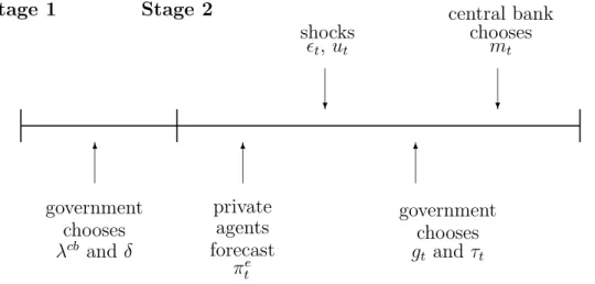
We characterize the strategic interaction between the government and the central bank as a two-stage non-cooperative game in which the structure of the model and the objective functions are common knowledge. In the ﬁrst stage, the government chooses the institutional parameters δ and λ^cb. The second stage is a Stackelberg game in which the government takes on the leadershiprole. In the second stage, the government and the monetary authority set their policy instruments, given theδ and λ^cb values determined at the previous stage. Private agents understand the game and form rational expectations for future prices in the second stage. Formally, the policy game can be described as follows:

Stage 1

The government solves the problem:

min

δ, λ^cb EL^g(g_t, m_t, δ, λ^cb) = E

1

2[π_t(g_t, m_t)−π]ˆ² − λ^g₁[y_t(g_t, m_t)]

+ λ^g₂

2 [(b−θ)y_t(g_t, m_t)−τ_t(g_t, m_t)]²

(9)

(10)

where L^g(g_t, m_t, δ, λ^cb) is (7) evaluated at (g_t, m_t, δ, λ^cb), and E is the expectations operator.

Stage 2

(i) Private agents form rational expectations about future prices π_t^e before the shocks u_t and _t are realized.

(ii) The shocks u_t and _t are realized and observed by the government and by the central bank.

(iii) The government choosesg_t, beforem_tis chosen by the central bank, to minimize L^g(g_t, m_t,δ,¯ λ¯^cb), where ¯δand ¯λ^cbindicates that these variables were determined in stage 1.

(iv) The central bank chooses m_t, taking g_t as given, to minimize L^cb(g_t, m_t,δ,¯ ¯λ^cb) =

(1−¯δ)

2 [π_t(g_t, m_t)−π]ˆ²−(1−δ)¯¯λ^cb[y_t(g_t, m_t)]

+ ¯δL^g(g_t, m_t,δ,¯ λ¯^cb) (10)

The timing of our two-stage game is illustrated in Figure 1.

Stage 1 Stage 2

✻

government chooses λ^cb and δ

✻

private agents forecast

π^e_t

❄

shocks

t, u_t

❄

central bank chooses

m_t

✻

government chooses g_t and τ_t

Figure 1: The Stages and Timing of the Policy Game

(11)

This game can be solved by ﬁrst solving the second stage of the problem for the optimal money supply and government expenditure policies withδand λ^cb ﬁxed, and then solving stage 1 by substituting the stage 2 results into (9) and minimizing with respect to δ and λ^cb. The equilibrium for the stage 2 leader-follower game is:

m_t(δ, λ^cb) = βπˆ

(β+γ) + (1−δ)β[β(φ−ηΛ)λ^g₂ + αγ(βη+γ)s²]λ^cb α(β+γ)[β(φ−ηΛ) +δΛ(βη+γ)]λ^g₂

+ δβ[βφ+γΛ)λ^g₁

α(β+γ)[β(φ−ηΛ) +δΛ(βη+γ)] − (1−γθs)u_t α(β+γ)

− (1−δ)βγs²(βη+γ)λ^g₁

(β+γ)[β(φ−ηΛ) +δΛ(βη+γ)]λ^g₂ − ^t

(β+γ) (11)

g_t(δ, λ^cb) = βπˆ

(β+γ) + (1−δ)β²[(φ−ηΛ)λ^g₂−αs²(βη+γ)]λ^cb α(β+γ)[β(φ−ηΛ) +δΛ(βη+γ)]λ^g₂

+ δβ[βφ+γΛ)λ^g₁

α(β+γ)[β(φ−ηΛ) +δΛ(βη+γ)] − (1 +βθs)u_t α(β+γ)

+ (1−δ)(βs)²(βη+γ)λ^g₁

(β+γ)[β(φ−ηΛ) +δΛ(βη+γ)]λ^g₂ − ^t

(β+γ) (12)

where

η = ∂m_t

∂g_t = −α²γβs² + δφΛλ^g₂

(αβs)² + δΛ²λ^g₂ (13)

φ = 1 +αβ−γθs (14)

Λ = 1 +αβ+βθs. (15)

Taking the mathematical expectation of both sides of (11) and (12) to obtain m^e_t andg_t^e, respectively, and substituting the result, together with (11) and (12), into (4) and (5) yields the reduced-form solutions forπ_tandy_tas functions of the institutional variables δ and λ^cb

π_t(δ, λ^cb) = ˆπ + (1−δ)β(φ−ηΛ)λ^cb + δ[βφ+γΛ]λ^g₁

α[β(φ−ηΛ) + δΛ(βη+γ)] (16)

(12)

y_t(δ, λ^cb) = −u_t

α . (17)

From (6), the reduced-form solution for τ_t is given by τ_t(δ, λ^cb) = (1−δ)βs(βη+γ)(λ^cb−λ^g₁)

[β(φ−ηΛ) + δΛ(βη+γ)]λ^g₂ − (b−θ)u_t

α . (18)

Substituting (16)–(18) into (9), the government’s stage 1 minimization problem can be expressed as

min

δ,λ^cb EL^g(δ, λ^cb) = 1 2

(1−δ)β(φ−ηΛ)λ^cb + δ[βφ+γΛ]λ^g₁ α[β(φ−ηΛ) + δΛ(βη+γ)]

₂

+ λ^g₂ 2

(1−δ)βs(βη+γ)(λ^cb−λ^g₁) [β(φ−ηΛ) + δΛ(βη+γ)]λ^g₂

₂

. (19)

Partial diﬀerentiation of (19) with respectλ^cb and δ yields the ﬁrst-order conditions

∂EL^g(δ, λ^cb)

∂λ^cb =

[(1−δ)β(φ−ηΛ)λ^cb+ δ[βφ+γΛ]λ^g₁](1−δ)β(φ−ηΛ) α²[β(φ−ηΛ) + δΛ(βη+γ)]²

− (1−δ)²(βs)²(βη+γ)²(λ^g₁−λ^cb) λ^g₂[β(φ−ηΛ) + δΛ(βη+γ)]² = 0

(20)

∂EL^g(δ, λ^cb)

∂δ =

(1−δ)β(φ−ηΛ)λ^cb+δ[βφ+γΛ]λ^g₁β[βφ+γΛ]

(λ^g₁−λ^cb){δ(1−δ)ΛΩ + (φ−ηΛ)} α²[β(φ−ηΛ) + δΛ(βη+γ)]³

− (1−δ)(βη+γ)(βs)²[βφ+γΛ]

{(βη+γ)−(1−δ)βΩ}(λ^g₁−λ^cb)² λ^g₂[β(φ−ηΛ) + δΛ(βη+γ)]³ = 0

(21) where Ω =∂η/∂δ.

(13)

It is evident that [β(φ−ηΛ) +δΛ(βη+γ)] = 0 is not a solution to the minimization problem. When [β(φ−ηΛ) +δΛ(βη+γ)]= 0, (20) and (21) yield, respectively, (22) and (23):

(1−δ)(φ−ηΛ)λ^g₂(1−δ)β(φ−ηΛ)λ^cb+δ[βφ+γΛ]λ^g₁

− (1−δ)²(βη+γ)²(αs)²β(λ^g₁−λ^cb) = 0 (22)

(1−δ)β(φ−ηΛ)λ^cb+δ[βφ+γΛ]λ^g₁(λ^g₁−λ^cb)

{δ(1−δ)ΛΩ + (φ−ηΛ)}λ^g₂

− (1−δ)(βη+γ)(αs)²β{(βη+γ)−(1−δ)βΩ}(λ^g₁−λ^cb)² = 0. (23) There are two real-valued solutions that satisfy the first-order conditions given above and which fall within the permissible range forδ.⁷ By inspection, it is apparent that (22) and (23) are both satisfied when δ = 1 and λ^cb = λ^g₁. This solution characterizes a central bank that is fully dependent. The second real-valued solution is δ = λ^cb = 0. In this case, the central bank is fully independent and exclusively concerned with the economy’s inflation performance.

The solution that yields the minimum loss for the government, as measured by the government’s loss function (7), can be identiﬁed by using (19) to compare the expected loss that would be suﬀered under the alternative institutional arrangements.

Substituting δ= 1 andλ^cb=λ^g₁ into (19) results in EL^g = (λ^g₁)²

2α² . (24)

Substituting δ=λ^cb = 0 into the right-hand-side of (19) yields

EL^g = 0. (25)

7Becauseηis a function ofδ, (23) is a quartic polynomial inδ. This polynomial has four distinct roots, of which only two are real-valued. Details of the complete solution set for the ﬁrst-order conditions may be found in Appendix1.

(14)

It is evident that when institutional arrangements are such that the government is the Stackelberg leader in the second stage policy game, the optimal central bank design, from society’s point of view, is one in which the central bank required to use monetary policy to achieve the government’s chosen inﬂation target and is granted full independence to do so. As we show in Appendix 2, central bank leadership does not provide as good a result from the government’s point of view, even ifthe government dictates the inﬂation target.

Our results show that when there is government leadership, society’s welfare, as measured by the inverse of (19), is maximized when the government appoints central bankers who are concerned only with the achievement of the mandated inﬂation target, and completely disregard the impact that their policies may have on output growth. However, our results also indicate that full central bank independence is beneﬁcial under more general conditions. Whenδ = 0, βη+γ = 0, and (19) is given by

EL^g = 1 2

λ^cb α

2

(26) for any arbitrary value of λ^cb, when δ= 0. Clearly, an independent central bank will always produce better results as long as it is more conservative than the government (λ^cb < λ^g₁), irrespective of the latter’s commitment to social equality (λ^g₂).

In deriving our results, we have assumed that the central bank has instrument independence but not target independence. Consequently, the fact that EL^g = 0 can be achieved by setting δ = λ^cb = 0 indicates that it is instrument independence which matters; and that target independence is ultimately irrelevant when there is government leadership. Neither target independence nor central bank leadership would reduce society’s expected loss to zero (see Appendix 2).

6. The Advantage of Government Leadership

6.1 Implications of the Theoretical Model

In Hughes Hallett and Weymark (2001), we show that if, in the second stage of

(15)

the game, government leadershipis removed so that monetary and ﬁscal policy are implemented simultaneously, then the government’s expected loss is given by

EL^g = 1 2

λ^g₁ α

₂

(αγs)² (αγs)² + φ²λ^g₂

. (27)

As long as the government has some commitment to social equality (i.e.,λ^g₂ = 0), (27) will always be smaller than the loss incurred when government leadershipis combined with a dependent central bank .

A more interesting question in this context is whether government leadership with an independent central bank generally produces better outcomes, from society’s perspective, than those obtained in the simultaneous move game. In the simultaneous move game, the solution to the government’s stage 1 minimization problem is

δ = βφ²λ^cbλ^g₂ + (αγ)²β(λ^cb−λ^g₁)

βφ²λ^cbλ^g₂ + (αγ)²β(λ^cb−λ^g₁) − φ[βφ+γΛ]λ^g₁λ^g₂.⁸ (28) The optimal degree of conservatism for an independent central bank in this type of game can be obtained by setting δ = 0 in (28) to yield:

λ^cb^∗ = (αγs)²λ^g₁

(αγs)²+φ²λ^g₂ (29)

It is straightforward to show that (26) is always less than (27) as long as

λ^cb < λ^g₁λ^cb^∗^1/2 (30)

It is also evident that λ^cb^∗ ≤ λ^g₁ for λ^g₂ ≥ 0. Consequently, government leadership with any λ^cb < λ^cb^∗ will produce better outcomes, from society’s point of view, than any simultaneous move game between the central bank and the government.⁹ This

8See Weymark (2001) for a full derivation of this result.

9Hughes Hallett and Weymark (2001) also show that λ^cb^∗ is the critical value that is relevant for comparing government leadership to any simultaneous move regime, including those withδ= 0.

This result follows from the substitutability betweenδ andλ^cb in (28).

(16)

is an important observation because many inﬂation targeting regimes, such as those operated by the Bank of England, the Swedish Riksbank, and the Reserve Bank of New Zealand, operate with government leadership; while several others, notably the European Central bank and the US Federal Reserve System, are better characterized as being engaged in a simultaneous move game with their governments.

Substituting δ = 0 and λ^cb into (16)–(18) shows exactly where the advantages of government leadershipcome from. We get

π_t = ˆπ, y_t = −u_t

α , τ_t = −(b−θ)u_t

α (31)

as the ﬁnal outcomes. By contrast, the optimal outcomes for the associated simultaneous move policy game are

π_t^∗ = ˆπ + α(γs)²

[(αγs)² + φ²λ^g₂] (32)

y_t^∗ = −u_t

α (33)

τ_t^∗ = γs(λ^cb^∗ −λ^g₁)

φλ^g₂ − (b−θ)u_t

α (34)

Comparing the two sets of outcomes we see that government leadership eliminates inflationary bias and therefore results in a lower rate of inflation. The optimal outcome under government leadershipis also characterized by higher taxes and therefore more income redistribution.¹⁰ Moreover, these improvements in inflation control and income distribution can be achieved with no loss in expected growth.

One of the central issues addressed in the policy coordination literature is whether there are institutional arrangements that yield Pareto improvements over the non- cooperative outcome.¹¹ When such institutions can be identiﬁed, they are viewed as

10Taxrevenues are lower under the simultaneous move game becauseλ^cb^∗< λ^g₁. Redistribution is positively related to the amount of taxrevenue because (b−θ)Ey^∗_t = 0, so thatτ_t^∗ determines the amount of income redistribution actually achieved.

11See, for example, Currie, Holtham, and Hughes Hallett (1989); Currie (1990); and Currie and Levine (1991).

(17)

a coordination device. In our model, government leadershipin the second stage of the policy game results in better outcomes for both policy authorities and is therefore an example of a rule-based form of policy coordination.¹²

6.2 Empirical Evidence

Whether or not the theoretical results we have obtained are of practical signiﬁcance is an empirical matter. In order to assess the magnitudes of the results we have obtained, we have computed the optimal degrees of conservatism and the associated expected losses under the simultaneous move and government leadership regimes for nine countries. The data we have used is from 1998, which is the year the Eurozone was created. The data itself, and its sources, are summarized in the appendix to this article.

Our sample of countries consists of those which have recently reformed their monetary policy frameworks with the explicit aim of securing lower and more stable inﬂation rates without damaging the prospects for growth, stability, or social equity.

The countries selected fall into three broad groups:

(a) Eurozone countries: France, Germany, and Italy

(b) Non-EMU countries with explicit inﬂation targets: Sweden, Switzerland, and the UK

(c) Inﬂation targeters outside the EU: Canada, New Zealand, and the US.

Each of these countries (the US excepted) has revised the statutes and the way in which the central bank is required to conduct monetary policy over the past ﬁve to ten years. In each case the creation of an independent central bank (whether fully independent or only instrument independent) has been the key feature of the reforms.

In the ﬁrst group, monetary policy is conducted at the European level and ﬁscal policy is conducted independently at the national level. Policy interactions in this groupcan be characterized in terms of a simultaneous move game with target as well

12See Currie (1990) for a discussion of the distinction between rule-based and discretionary, orad hoc, forms of policy coordination.

(18)

Table 1

Losses under Government Leadershipand Simultaneous Moves Full Government Simultaneous Growth Rate Dependence Leadership Moves Equivalents

δ = 1 δ = 0 δ = 0 Lost

λ^cb=λ^g₁ λ^cb= 0 λ^cb =λ^cb^∗ %

France 5.78 0.00 0.0125 1.26

Germany 16.14 0.00 0.0079 0.79

Italy 1.28 0.00 0.0116 1.16

Sweden 4.51 0.00 0.0098 0.98

Switzerland 4.79 0.00 0.0251 2.51

UK 3.37 0.00 0.0113 1.13

Canada 12.50 0.00 0.0265 2.65

New Zealand 8.40 0.00 0.0104 1.04

USA 6.47 0.00 0.0441 4.41

as instrument independence. The second group of countries has adopted explicit, and usually publicly announced, inflation targets. Central banks in these countries have been granted a high degree of instrument independence. The government either sets, or helps set, the inflation target value. In each case the government has adopted longer term (supply side) fiscal policies, leaving active demand management to monetary policy. These are clear cases in which there is government leadership, with instrument independent for the central bank.¹³ Of the countries in the third group, New Zealand and Canada can also be described as explicit inflation targeters with government leadership. The US, although not an explicit inflation targeter, is included in this group as a point of comparison because of the success with which monetary policy has been employed in the US over the past decade.

The results of our calculations are reported in Table 1. The ﬁrst column in this

13Switzerland is included in this group on the basis of the inﬂation targeting changes made after 1999. See Rich (2000) for a detailed analysis of the inﬂation targeting process in Switzerland.

(19)

table shows the losses that would be incurred with a fully dependent central bank;

these losses are identical under both regimes. Column two reﬂects the losses that would be incurred under government leadershipwith a fully independent central bank that directs monetary policy exclusively towards the achievement of the inﬂation target (i.e., with δ =λ^cb = 0). The third column gives the minimum loss associated with simultaneous decision-making in stage two of the policy game.¹⁴

Evidently, complete dependence is extremely unfavourable for all countries. How- ever, the magnitude of the loss varies considerably from country to country. The losses in column three, relative to those in column 2 appear to be relatively small when measured in terms of raw welfare units. However, when these losses are con- verted into “growth rate equivalents”, we ﬁnd that there are signiﬁcant losses associated with institutional arrangements in which government leadershipis absent.

The growth rate equivalents reported in the last column of Table 1 were obtained using a standard technique borrowed from the coordination literature.¹⁵ Specifically, we have computed the marginal rates of transformation around each government’s indifference curve to find the change in output growth, dy_t, that yields the welfare loss given in column four when all other policy variables are held at their optimized values. Formally, we use (7) together with certainty equivalence to obtain

dy_t = (dEL^g_t)

[λ^g₂{(b−θ)y_t−τ_t}(b−θ)−λ^g₁]. (35) The minimum value of dy_t is attained when the taxτ_t grows at the same rate as the redistribution target (b−θ)y_t. These minimum output losses are reported in column four.

The values in column four show that the losses associated with simultaneous decision-making are equivalent to permanent reductions of 1–2 percent in the long term growth rate of national income. These are signiﬁcant losses and are roughly

14The losses reported in column 3 were calculated using λ^g₁ = 1 and λ^g₂ = 0.5 for each of the countries in the sample as in Hughes Hallett and Weymark (2001).

15See, for example, Currie et al (1989), Nolan (2002), and Oudiz and Sachs (1984).

(20)

Table 2

Central Bank Conservatism –λ^cb

Government Simultaneous Leadership Moves optimal upper optimal

value bound value

France 0.00 0.0466 0.00217

Germany 0.00 0.0221 0.00049

Italy 0.00 0.0952 0.00906

Sweden 0.00 0.0467 0.00218

Switzerland 0.00 0.0725 0.00525

UK 0.00 0.0579 0.00335

Canada 0.00 0.0458 0.00212

New Zealand 0.00 0.0351 0.00123

USA 0.00 0.0826 0.00682

equivalent to all the gains that might be expected from international policy coordination (Currie et al, 1989), or from introducing the single currency in Europe (EC, 1990).

In Table 1 we have compared the losses associated with government leadership and simultaneous decision-making when the central banking institutions are optimally conﬁgured within each regime. However, (30) indicates that the government leadership regime does not need to be optimally conﬁgured in order to produce outcomes that are superior to those achieved in the simultaneous move regime. In Table 2, we provide estimates of the lowest degree of central bank conservatism (i.e., the highest value of λ^cb) for which government leadershipcombined with central bank independence will dominate the optimal simultaneous-move regime. Our calculations show that, compared to the optimal simultaneous-move regime, considerably less central bank conservatism is required to produce good economic outcomes when there is government leadershipin policy formation. For Germany, the losses would be lower

(21)

under government leadershipwith λ^cb values as much as 50 times larger than under an optimal simultaneous-move regime. In the case of Italy, government leadership is beneﬁcial for λ^cb values of upto 10 times larger than under an optimally conﬁg- ured simultaneous-move regime. The remaining six countries fall in between these two extremes. In all cases, the degree of central bank conservatism required under simultaneous decision-making is at least an order of magnitude greater than what is needed when there is government leadership.

The implication of these results is that instrument independence, coupled with government led ﬁscal policies, allows policy makers a great deal more room for manouevre than do regimes that are characterized by a combination of target independence and simultaneous policy moves. Government leadership expands the fea- sible policy space in that both the central bank and the government can contemplate a wider range of policies to suit their own objectives and still expect to get better outcomes, from society’s point of view, than in other regimes. Conversely, a government leadershipregime is likely to be less sensitive to any variations in the transmission parameters, savings ratios, or targets for social equality that may appear around the economic cycle, or as new governments come into oﬃce. This last point may prove to be the greater advantage in practical applications.

7. Conclusion

In this article, we have developed a model of monetary delegation in which the government plays a leadership role. We find that when the government has the first-mover advantage in formulating fiscal policy, society’s well-being (as we have defined it) is maximized by appointing a central banker whose only concern is the achievement of the government-mandated inflation target.

Our theoretical results show that government policy leadership, coupled with a fully independent, inﬂation-oriented central bank, will lead to a better economic performance, from society’s point of view, than a simultaneous move game between the central bank and the government. In comparing the optimal economic outcomes that

(22)

can be achieved under each of the two regimes, we ﬁnd that government leadership results in Pareto improvements across all objectives for all players. This suggests that the improved outcomes obtained under government leadership come from the greater (implicit) coordination that this regime generates between the two independent policy authorities.

Our empirical analysis indicates that the benefits of government leadership are large enough to allow policy makers to achieve good outcomes with a much wider range of policies than in the simultaneous move regime. Moreover, because the success of the leadershipregime is less sensitive to the precise choice of the degree of conservatism, it provides some protection against the impact of variations in transmission parameters or social objectives on economic outcomes. Our results are of particular significance for countries like the UK and Sweden, who must decide whether the benefits of joining the European Monetary Union are sufficient to justify the cost of giving up monetary sovereignty and government leadershipin policy formation.

References

Barro, R.J. (1981) “Output Eﬀects of Government Purchases,” Journal of Political Economy 89, 1086-1121.

Barro, R.J. and D.B. Gordon (1983) “Rules, Discretion, and Reputation in a Model of Monetary Policy,” Journal of Monetary Economics 12, 101-21.

Currie, D.A. (1990) “International Policy Coordination,” in D.T. Llewellyn and C.

Milner (eds.) Current Issues in International Monetary Economics, Macmillan, London, 125-48.

Currie, D.A., G. Holtham, and A. Hughes Hallett, (1989) “The Theory and Practice of International Economic Policy Coordination: Does Coordination Pay?” in R.

Bryant, D. Currie, J. Frenkel, P. Masson, and R. Portes (eds.) Macroeconomic Policies in an Interdependent World, International Monetary Fund, Washington DC.

(23)

Currie, D.A. and P. Levine (1991) “The International Coordination of Monetary Policy – A Survey,” in C.J. Green D.T. Llewellyn (eds.) Surveys in Monetary Economics, Vol. 1, Cambridge MA and Oxford, Basil Blackwell.

Dixit, A.K. and L. Lambertini (2001) “Fiscal Discretion destroys Monetary Commit- ment,” Unpublished Manuscript, Department of Economics, Princeton Univer- sity.

Fischer, S. (1995) ”Central Bank Independence Revisited,”American Economic Re- view 85, 201-6.

Hughes Hallett, A. (1998) “When Do Target Zones Work? An Examination of Ex- change Rate Targeting as a Device for Coordinating Economic Policies” Open Economies Review 9, 115-38.

Hughes Hallett, A. and D.N. Weymark (2001) ”The Cost of Heterogeneity in a Mone- tary Union,” Discussion Paper No. 3223, Center for Economic Policy Research, London; Working Paper No. 01-W28, Department of Economics, Vanderbilt University, <www.vanderbilt.edu/econ>.

Lucas, R.E. (1973) “ Some International Evidence on Output-Inﬂation Trade-Oﬀs,”

American Economic Review 63, 326-34.

Lucas, R.E. (1972) “ Expectations and the Neutrality of Money,” Journal of Eco- nomic Theory 4, 103-24.

McCallum, B.T. (1989) Monetary Economics: Theory and Policy, Macmillan, New York.

Rich, G. (2000) “Monetary Policy Without Central Bank Money: A Swiss Perspec- tive,” International Finance 3, 437-469.

Nolan, C. (2002) “Monetary Stabilization Policy in a Monetary Union: Some Simple Analysis,” Scottish Journal of Political Economy, forthcoming.

Oudiz, G. and J. Sachs (1984) “Macroeconomic Policy Coordination Among the In- dustrial Economies,” Brookings Papers on Economic Activity 1, 1-64.

Taylor, J.B. (1993) Macroeconomic Policy in a World Economy: From Econometric Design to Practical Operation, W.W. Norton and Company, New York.

(24)

Turner, D., and E. Seghezza (1999) “Testing for a Common OECD Phillips Curve,”

Working Paper No. 219, Economics Department, OECD, Paris.

Weymark, D. N. (2001) “Inﬂation, Income Redistribution, and Optimal Central Bank Independence,” Working Paper No. 01-W02R, Department of Economics, Van- derbilt University. <www.vanderbilt.edu/econ>.

Appendix 1 Solutions to (22) and (23)

The ﬁrst-order condition (23) can be written as a quartic polynomial in δ. As a consequence, there are four solutions that simultaneously satisfy (22) and (23). By inspection, it is apparent that one of these solutions is δ = 1 and λ^cb = λ^g₁. When δ= 1 and λ^cb =λ^g₁, the ﬁrst order conditions can be written

(φ−ηΛ)λ^g₂(1−δ)β(φ−ηΛ)λ^cb + δ[βφ+γΛ]λ^g₁

− (1−δ)(βη+γ)²(αs)²β(λ^g₁−λ^cb) = 0 (A.1)

δ(1−δ)Λ∂η

∂δ + (φ−ηΛ)(1−δ)β(φ−ηΛ)λ^cb + δ[βφ+γΛ]λ^g₁λ^g₂

− (1−δ)(βη+γ)(αs)²β

(βη+γ) − (1−δ)β∂η

∂δ (λ^g₁−λ^cb) = 0.

(A.2) But (A.2) can be expressed as

(A.1) + δ(1−δ)Λ∂η

∂δ

(1−δ)β(φ−ηΛ)λ^cb+δ[βφ+γΛ]λ^g₁λ^g₂ + (1−δ)²(βη+γ)∂η

∂δ(αβs)²(λ^g₁−λ^cb) = 0. (A.3) Consequently, when δ = 1 and (A.1) is satisﬁed, (A.2) becomes

δΛ(1−δ)β(φ−ηΛ)λ^cb+δ[βφ+γΛ]λ^g₁λ^g₂

+ (1−δ)(βη+γ)(αβs)²(λ^g₁ −λ^cb) = 0. (A.4)

(25)

Replacing η with (13) yields (φ−ηΛ) = α²βs²[βφ+γΛ]

(αβs)²+δΛ²λ^g₂ and (βη+γ) = δΛ[βφ+γΛ]λ^g₂

(αβs)²+δΛ²λ^g₂. (A.5) It is evident that (βη+γ) = 0 when δ = 0. Hence δ =λ^cb = 0 is one solution that satisﬁes (A.1) and (A.4).

The remaining potential solutions can be found by substituting (A.5) into (A.4) and solving for δ (under the assumption that δ = 0 andδ= 1). We obtain:

δ² = −(αβs)²

Λ²λ^g₁λ^g₂ . (A.6)

Consequently, there are only two real-valued solutions that satisfy the ﬁrst-order necessary conditions: (i) δ= 1 and λ^cb =λ^g₁, and (ii) δ=λ^cb = 0.

Appendix 2 Central Bank leadership

This appendix summarizes the results obtained when the central bank, rather than the government, is the Stackelberg leader in the second stage of the policy game. Because a central bank that plays a leadership role is almost certain to have target independence, we express the objectives of the central bank as follows:

L^cb_t = 1

2(π_t−πˆ^cb)² −(1−δ)λ^cby_t−δλ^g₁y_t+δλ^g₂

2 [(b−θ)y_t−τ_t]² (A.7) where we allow the central bank’s inflation target ˆπ^cb to differ from the government’s inflation target ˆπ.

When the central bank has full target independence and is the Stackelberg leader, the reduced-form solutions for π_t,y_t, and τ_t are:

π_t = [(β+µγ)φπˆ^cb + δγ(Λ−µφ)ˆπ

(β+µγ)φ + δγ(Λ−µφ) + (1−δ)(β+µγ)φλ^cb α[(β+µγ)φ + δγ(Λ−µφ)]

+ δ[βφ+γΛ]λ^g₁

α[(β+µγ)φ + δγ(Λ−µφ)] (A.8)

(26)

y_t = −u_t

α (A.9)

τ_t = αγs(β+µγ)(ˆπ−πˆ^cb) [(β+µγ)φ + δγ(Λ−µφ)]λ^g₂

+ (1−δ)γ(β+µγ)s(λ^g₁−λ^cb)

[(β+µγ)φ + δγ(Λ−µφ)]λ^g₂ − (b−θ)u_t

α (A.10)

whereµ = ∂g_t

∂m_t = −α²βγs² + φΛλ^g₂ (αγs)² + φ²λ^g₂ .

Substituting (A.8)–(A.10) into the government’s loss function (7) and diﬀerenti- ating with respect toλ^cb and δ yields the necessary ﬁrst-order conditions:

∂EL^g_t

∂λ^cb = 0

⇒ (1−δ)φλ^g₂−αΓφ(ˆπ−πˆ^cb) +φ(1−δ)Γλ^cb+δ[βφ+γΛ]λ^g₁

− (αγs)²Γ(1−δ)α(ˆπ−πˆ^cb) + (1−δ)(λ^g₁−λ^cb) = 0

(A.11)

∂EL^g_t

∂λ^cb = 0

⇒ φλ^g₂ΓΣ−α(β+µγ)φ(ˆπ−πˆ^cb) +φ(1−δ)Γλ^cb+δ[βφ+γΛ]λ^g₁

−(αγs)²Γ²Σα(ˆπ−πˆ^cb) + (1−δ)(λ^g₁−λ^cb) = 0

(A.12) where

Σ = [βφ+γΛ](λ^g₁−λ^cb) + αγ(ˆπ−πˆ^cb)(Λ−µφ) Γ = (β+µγ).

There are two solutions that satisfy both of the ﬁrst-order conditions given above.

By inspection, it is apparent that (A.11) and (A.12) are both satisﬁed when δ = 1 and Γ = 0. When 0 ≤δ <1 and Γ = 0, then (A.11) and (A.12) imply the following relationshipbetweenδ and λ^cb

δ = (β+µγ)φ²λ^cbλ^g₂ + (αγs)²(λ^cb−λ^g₁) − α[φ²λ^g₂+ (αγs)²](ˆπ−πˆ^cb) (β+µγ){φ²λ^cbλ^g₂ + (αγs)²(λ^cb−λ^g₁)} − φ[βφ+γΛ]λ^g₁λ^g₂ .

(A.13)