GP Multiscale Thesis - AURA - Alfred University

INTRODUCTION

Motivation

The MT method is included in such well-known simulation programs as GULP.6 Although this method can be used to investigate the general characteristics of defects, it lacks sufficient interaction with operating load conditions, the model is oversimplified and suffers from small model sizes that struggle to simulate defect nucleation in realistic processes. Recently, discrete dislocation analysis confirms experimental results that the flow strength of polycrystals depends on grain size.7 This type of analysis enables the interpretation of plastic mechanisms, as well as size and surface effects, for free-standing FCC thin films.8 Based on continuum dislocation theory, the analysis can also indicate typical material behavior such as the Bauschinger effect.9,10 The length scale effect of plasticity is incorporated through.

Classification of Multiscale methods

Hierarchical

Later in the 1990s a method using the sinusoidal Frenkel distribution25,26 for the shear stress along the slip plane ahead of the crack tip was proposed by Peierls27 and Nabarro (PN). Even with this advance the PN model has a shortcoming based on the transformation of the atomic behavior in the continuum representation and thus the model does not give the best results for the calculated dislocation slip energy.28 it happens that in this case the Class II RT model can be improved with an atomistically based class I model that can find the constitutive equation required by the RT model.29,30 Cleri et al.

Concurrent

A well-known Class II continuum model that predicts the brittle to ductile transition based on a competition between the loss of atomic cohesion and the release of crack tip dislocations, this model is known as the Rice-Thomson (RT) model.24 The difficulty with this model is the acquisition of the critical energy release from the sliding events. Most existing simultaneous multiscale methods do not show truly seamless transitions of key variables such as strain, motion and force at the scale interface.36 The transition problem is caused by the incompatibility between materials on both sides of the scale interface; the atomistic scale has nonlocal behavior while the continuum has local behavior.

Figure 1. Example of DC interface with atoms. 31

Atomistic-based multiscale analysis, Class-I

The latter has been used to investigate the individual sliding behavior of dislocations and the plastic slip behavior at the macroscale in single-crystal BCC metals. When dislocation multiplication occurs, they move toward the interior of the model and cross shell interfaces, so the accuracy of dislocations smoothly crossing the shell interface is essential.

Inadequacies and Existing Needs

METHODOLOGY OF THE ATOMISTIC-BASED MULTISCALE

The Generalized Particle (GP) Method

Material property scale independence
Scale interfaces
Surface corrections
Scale duality

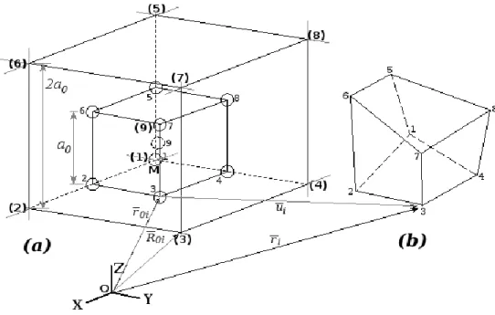
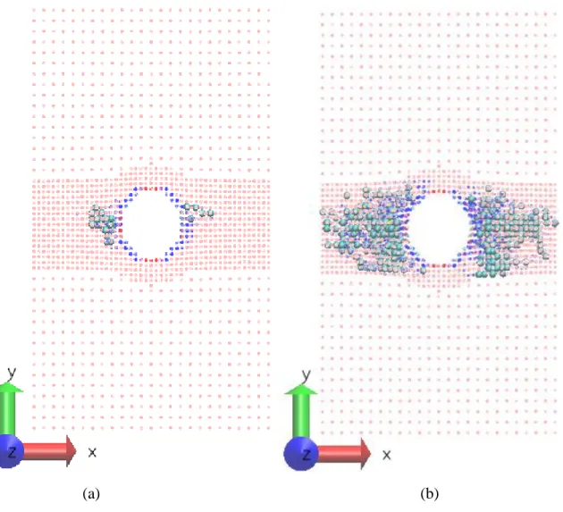
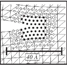
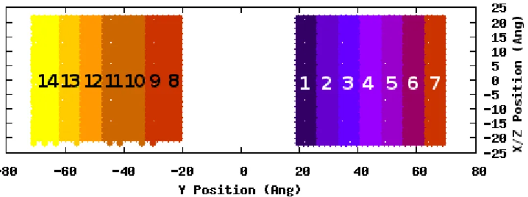
In this case the first definition will be used around the edges of the model. This figure shows the CN of the atoms in the central symmetric plane of the model (i.e. near y=0).

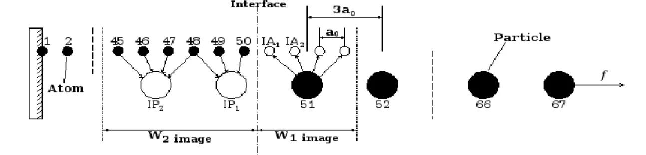
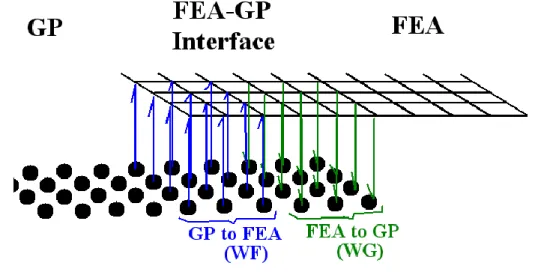
Figure 2. A 1D example model, exemplifying the scale interface and imaginary domains

Linking GP with FEA

Advantages of the GP-FEA Methodology
Model Structure and Design of Coupling subsystems
The “Bottom-Up” and “Top-Down” iteration bridging scheme
Numerical Algorithms

This is normal because the determination of the FE node positions in the WF domain is controlled by a relaxation process of the WG-GP subsystem. NI) is the ID number of a generic node and NI – the total number of FE nodes in the WF domain.

Figure 15. Schematic of the four main domains of a simple GP-FEA model. From the inner region to the outside in an ascending order: The GP domain, the WF and WG domains and the FEA domain

Shortcomings

This is natural since the WG-GP calculation to determine FE node positions for the WF-FEA subsystem BC is mainly a relaxation process to make the system equilibrate.

Summary

ACCURACY VERIFICATIONS OF ATOMISTICALLY-BASED

Introduction

According to this definition, most of the existing multiscale methods belong to the DC methods. Specifically, the behavior of the continuum on one side of the scale interface is local, but that of atoms on the other side is nonlocal in nature.

Model Development

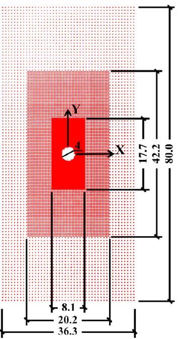
GP Hole Model development

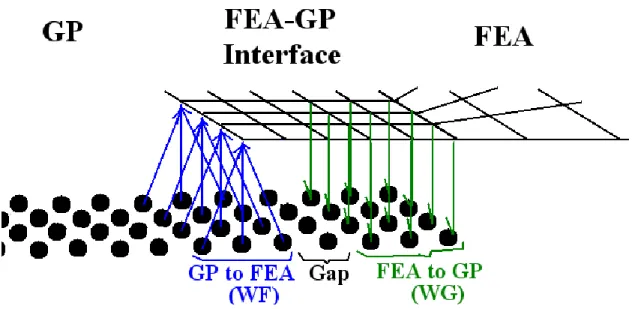
GP--FEA interface design

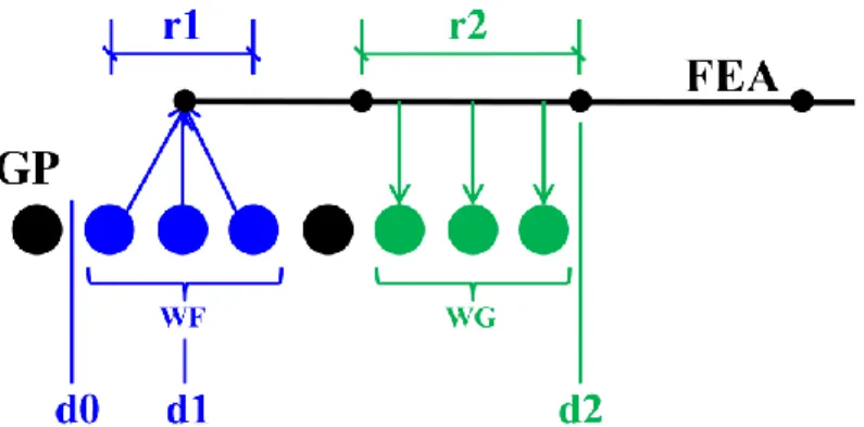
The particles in the WF average their positions to determine the position of the FE node, which is inside r1 in the WF domain. The size of the finite element in the interface should be uniform with respect to the size of the boundary radius between the particles and gradually increase further away from the GP domains.

FEA Mesh generation

After this separate equilibration, the FEA mesh is connected to the GP model for the loading procedure. Since the element size at the interface is designed to have an edge length equal to the cut-off radius between the particles, this will create two FE elements that overlap the GP model along the normal direction of the inner FE boundary .

Verification of the GP and GP-FEA multiscale methods with Elasticity Solutions for a

The scheme for the comparison of atomistically- based simulation with a continuum

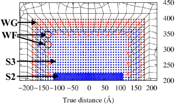
Verification of the GP and GP-FEA multiscale methods with Elasticity Solutions for a plate with a central hole under tensile loading. From that file one extracts the average displacement values of each of the specified cylinders.

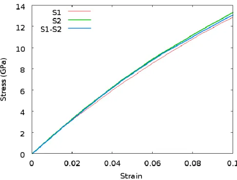
Result comparison for pure GP and GP-FEA model

Comparison of the 2% strain displacement of the obtained angular displacement and the calculated formulas 𝑢𝜃 and radial displacement 𝑢𝑟 along a circle of radius 8 nm in the first quadrant for a single crystal of iron. Comparison of 3% strain displacement of obtained angular displacement and calculated formulas 𝑢𝜃 and radial displacement 𝑢𝑟 along a circle of radius 8 nm in the first quadrant for a single crystal of iron.

Figure 19. Discontinuous WF domain design and its relation with high-scale particles and the WG domain for the GP-FEA model

Summary and Conclusions

ACCURACY VALIDATION WITH LEFM SOLUTION AT CRACK-TIPS

GP-FEA Model Design

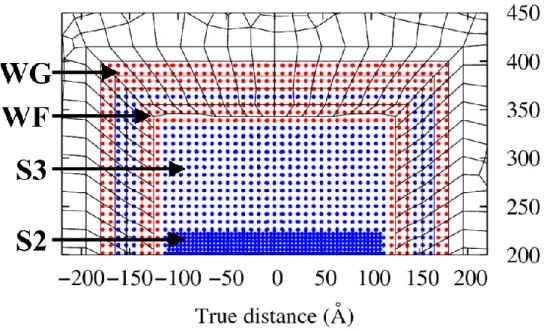
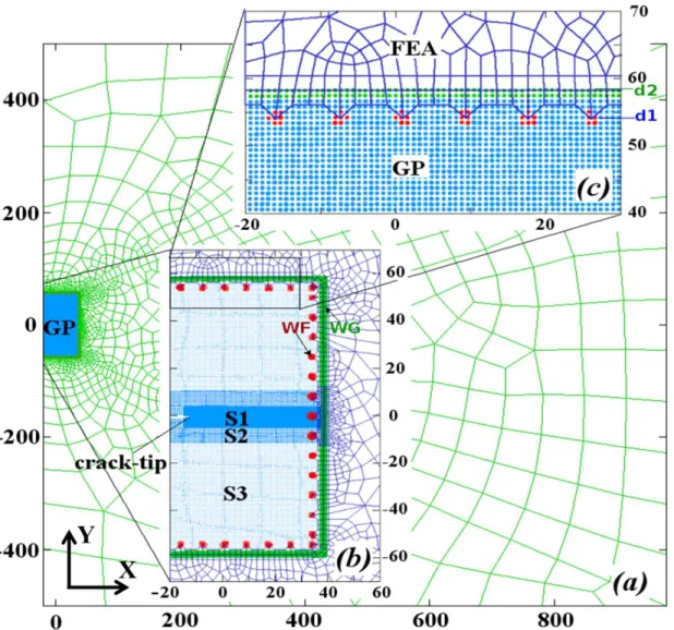
24b, the GP model consists of three particle scales representing an iron plate with an edge crack. Separate red dots indicate the WF domain, the narrow green band surrounding the GP model is the WG domain.

Figure 24. Schematic of a micrometer-size GP-FEA model with an embedded 60×120×4.5 nm 3 three-scale GP model for a thin plate with an edge crack, where the unit is nm

Comparison between LEFM solutions and GP-FEA simulation results for the crack-

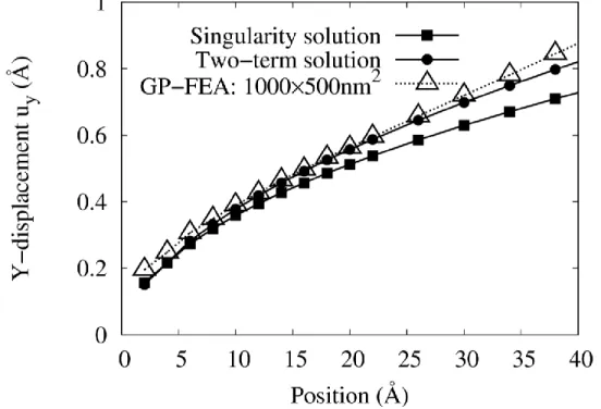
LEFM singularity solution and two-term solutions of crack-tip displacement field

Comparison between LEFM solutions and GP-FEA simulation results for crack tip displacement. 22) defines the stress per atom. In order to obtain the appropriate continuum voltage, a further averaging of the volume occupied by these atoms must be performed.

Comparison between atomistically-based multiscale simulation with both LEFM

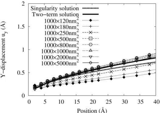
Therefore, in the next section we will mainly show the comparison of simulation results with the two-term LEFM solution. Comparison of radial displacement between GP-FEA simulation results with LEFM solutions along the circle of R = 15 Å in the first quadrant.

Figure 26. Y-Displacement comparison between results of GP-FEA simulation with LEFM solutions along the Y-axis

Model size effects on numerical results of displacement distribution near crack-tip in

Model size effects on the radial displacement component, ur, along the circle of R = 15 Å in the first quadrant. In that case, if the model size is small, the stress field near the crack tip will be seriously affected.

Figure 29. Effects of model size, L y , on the displacement component u y for the location along the Y-axis near the crack-tip within 2 to 40 Å

Summary and discussions

APPLICATION IN CRACK PROPAGATION

Simulation Model and Methods

The model used for the crack propagation simulations was essentially the same as described in Chapter IV. Refer to the figure in Chapter IV of the GP-FEA model as the GP model and the interface design are the same.

Crack Propagation Results via GP-FEA

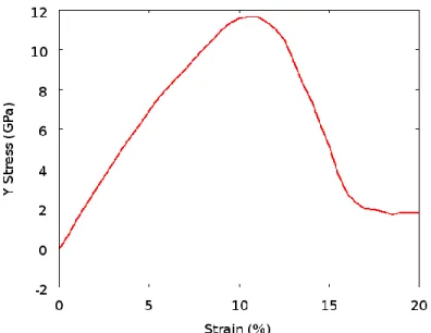
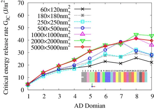
Fracture Energy

Notice how smaller models generally have lower critical energy release rates than larger models. 34 showing the critical level of energy release, GIC for local domains 5 and 6, showing a strong convergence trend.

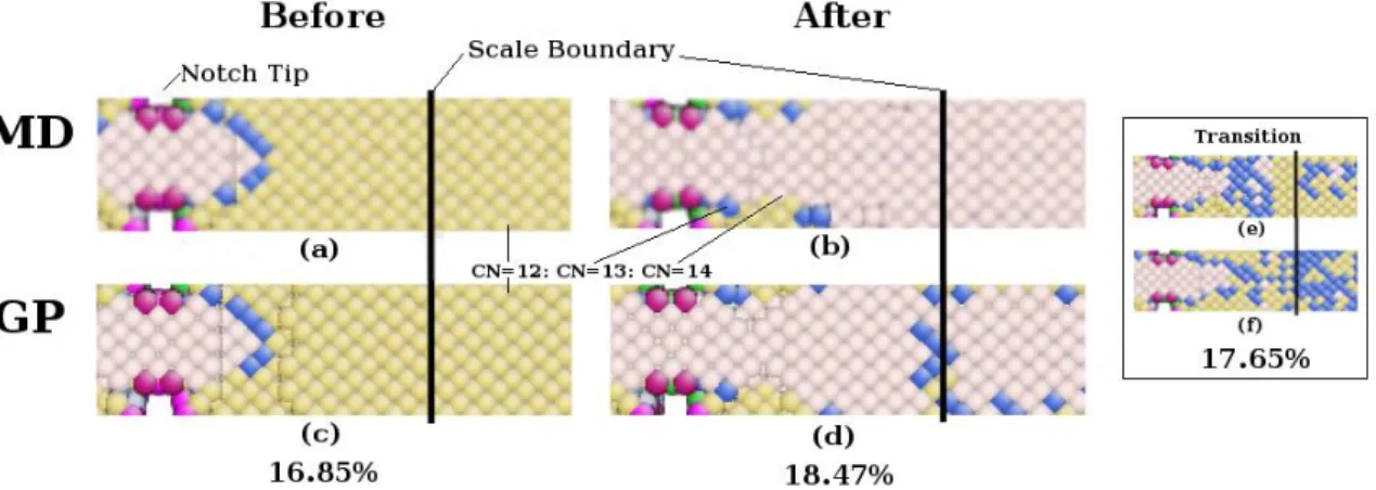
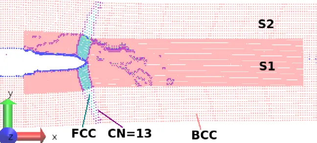
Figure 33. Energy G IC distribution during cracking the local domains.

Crack-Tip Phase Transformation

This indicates that the GP shell interface does not strongly inhibit the growth of the FCC phase. Smaller model sizes do not cause the FCC phase as quickly as the larger models do.

Figure 37. Example of crack-tip phase configuration for the 1 micron sized model.

Conclusion

APPLICATIONS IN IMPACT

GP Model for Wave Propagation

For the dynamic case, the new atoms, after dissolution, will have to be assigned the correct velocities and accelerations, in the same way as they are assigned positions in the deformation field. In the same way that position is determined, their speed and acceleration are also determined.

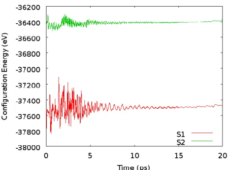
Figure 40. Impact model configuration, each numbered rectangle was individually monitored for stresses and energies and was later used as an Auto-Duality domain

MD Results for Wave Propagation

Scale-2 Results for Wave Propagation

It can also be seen from the period of the waves that the wave speed in scale-2 is twice as great as the atomistic model. This corresponds to the same acceleration that an atom would feel due to the greater mass of the particle.

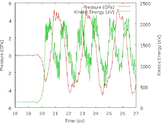
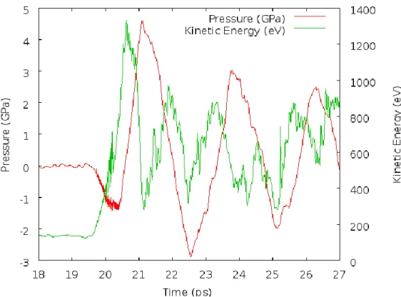
Figure 43. Kinetic and Potential energy evolution for the pure Scale-2 model at the time of impact

Auto-Duality Results for Wave Propagation

Kinetic energy and pressure evolution for the auto-duality model at the moment of impact. The auto-duality model still suffers from increased kinetic energy due to the surface adhesion at scale 2, albeit to a lesser extent due to the dissolution.

Figure 46. Kinetic energy and Pressure evolution for the auto-duality model at the time of impact

Summary and Recommendations

PARTICLE-BASED MULTISCALE ANALYSIS PROGRAM (PMAP)

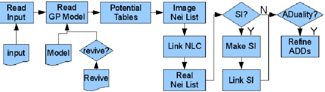
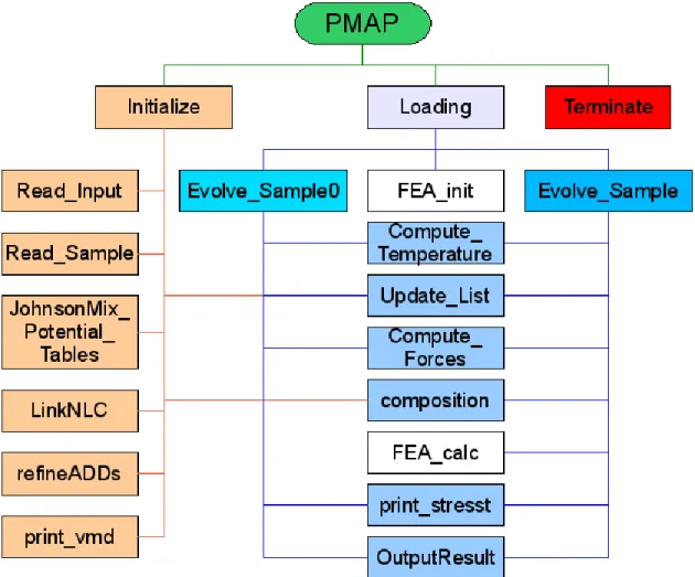
Functionality, constitution and flow charts of three basic processes of PMAP

Initialization Process

Neighbors that are included in the lists are of adjacent criteria that are not of the same criteria. When NLCs are created, all real atoms and particles are given new Verlet neighbor lists containing atoms and particles of the same range.

Equilibration Process

The system temperature is calculated at this point in preparation for a possible thermostat procedure. This works because all particle positions are normalized to the simulation box size, so they are essentially a function of the box size.

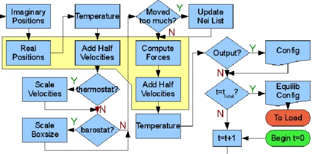
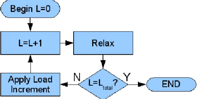
Loading Process

These forces provide new accelerations to be used in the second half of the Verlet velocity algorithm. At the end of the FEA calculation, it sends new interpolated positions of the WG particles to the relaxation process which uses them as a fully fixed boundary layer.

Figure 51. General flow of the GP load process.

Constructions and Executions

Post-processing

This method assumes that the strain gradient of the particle domain is the same as that of the degraded domain. As mentioned in Section VII.B.3, the charging process uses a relaxation procedure that is almost identical to the equilibration process.

CONCLUSIONS AND RECOMMENDATIONS

Conclusions

Therefore, it is essential to investigate the effects of model size and select the smallest model size necessary to meet the accuracy requirement. Varying the size of the model and comparing the behavior with the LEFM solution will quantitatively show the size effect.

Recommendations for Future Work

Cormack, "Molecular Dynamics Studies of Stress-Strain Behavior of Silica Glass under a Tensile Load," Chem. Cormack, "Molecular Dynamics Studies of Stress-Strain Behavior of Silica Glass Under a Trækbelastning," Chem.

USUAL MOLECULAR DYNAMIC FEATURES

Reading EAM Tables
Damped Shifted Coulomb Potential (DSC)
Simulation Revival
Periodic Boundary Conditions (PBC) using Verlet Neighbor Lists
Barostat (NPT)

First, the type of interaction; this is an integer defined at the beginning of the simulation. The second is to ensure that atoms close to the boundary can 'sense' the atoms on the other side; essentially, the force interactions must also be refolded.

Figure 53. The Ewald sum (A) replicates the simulation box infinitely. Radial cutoff methods (B) should be used for amorphous and geometrically unique systems[3]

GP FEATURES

Automatic Duality Domains (ADD) with stress and energy (internal duality)

This is the average position of all the NLC constituents, the negative of which is the error vector, errvect, line 4790. It searches through all ADDomains' maximum VM loads and compares it to the voltage range specified in the input file.

Link GP with FEA

This domain is inside the GP model and calculates the GP position average in the WF domain to assign FE nodes. Line 414 of the FEA code contains a routine that determines which element the WG particles are in.

Figure 56 shows that the inner layer (WF) directly modify the nodes that they are connected to, and the outer layer (WG) is defined by the FE nodes

Using local/scale BoxSizes for Verlet neighbor Lists to save memory in large models

MODEL DEVELOPMENT

GP model development program

The next line is the full domain of the block in the format a, x-left, x-right, y-back, y-forward, z-bottom, z-top. Where the first two parameters are the X and Z coordinates and the third is the radius of the cylinder.

Nano-structure generation

Lines 533-536 specify the ranges for the a and b axes for cutting and milling holes. These two domains would be two large elliptical grains that are clearly not part of the nanostructure being created.

External Decomposition (blind) versions: 2W 3, 5, 6one

This decomposition process is designed to increase the “data resolution” of the model by interpolating positions for the particle's constituent atoms. When finding these particles, the initial configuration is used because of the simplicity of using a regular structure.

Figure 60. Distance ratios are the same for the atom 'a' as for the particles.

Delete duplicate positions within a cutoff: delMDdup & delMD3dup

Considerations when designing very large micron scale models

These intermediate scales should ideally be greater than or equal to the size of the cutoff radius of the scale above, so that the higher scale's imaginary domain can fit inside when it is of an ideal size. The program to generate such a large model must be the model generation program described in Appendix C.1.

FE Mesh input file for the GP-FEA simulation

In this code, NMPC=0 because only the displacement BC is used, no data is used in this line. The last line of the comment specifies the FEA tolerance value to which the GP-FEA interface should converge, and the second number (e.g. number 19) is the maximum allowable number of iterations of the GP-FEA interface, km, after which the model will load regardless of whether the interface converged or not.

THE PARTICLE-BASED MULTISCALE ANALYSIS PROGRAM (PMAP)

PMAP Structure: Subroutines and functions

8 DomainCenter Returns the center position of the specified domain 9 full angle Returns the angle from the x-axis to vector, v. 13 Initial_Printout Prints information about the run parameters on standard output 14 Evolve_Sample0 Equilibration procedure; time evolution of the system.