G ROUND P ENETRATING R ADAR FOR
E NVIRONMENTAL A PPLICATIONS
Rosemary Knight
Department of Earth and Ocean Sciences, University of British Columbia, Vancouver, Canada1
Key Words geophysics, hydrogeology, contaminant transport, dielectric properties
■ Abstract Ground penetrating radar (GPR) is a near-surface geophysical technique that can provide high resolution images of the dielectric properties of the top few tens of meters of the earth. In applications in contaminant hydrology, radar data can be used to detect the presence of liquid organic contaminants, many of which have dielectric properties distinctly different from those of the other solid and fluid components in the subsurface. The resolution (approximately meter-scale) of the radar imaging method is such that it can also be used in the development of hydrogeologic models of the subsurface, required to predict the fate and transport of contaminants. GPR images are interpreted to obtain models of the large-scale architecture of the subsurface and to assist in estimating hydrogeologic properties such as water content, porosity, and permeability. Its noninvasive capabilities make GPR an attractive alternative to the traditional methods used for subsurface characterization.
INTRODUCTION
Ground penetrating radar (GPR) is a geophysical method that can provide high resolution three-dimensional images of the subsurface of the earth. Advances in radar technology over the past 10 to 15 years have led to its widespread use for imaging the top tens of meters of the earth. Digital radar systems are now available with a range of capabilities and are used for many varied applications including the assessment of groundwater resources, mineral exploration, archaeological studies and, as is the focus of this review, environmental applications.
The environmental application in which the use of GPR is most likely to lead to significant improvements in the currently practiced methodologies is in the field of contaminant hydrology. Locating and predicting the fate and transport of contaminants in the subsurface requires an accurate model of the physical,
1Current Address: Geophysics Department, Stanford University, Stanford, California 94305; e-mail: [email protected]
0084-6597/01/0515-0229$14.00 229
Annu. Rev. Earth Planet. Sci. 2001.29:229-255. Downloaded from www.annualreviews.org by University of Sydney on 04/10/13. For personal use only.
chemical, and biological properties of the earth. While traditional methods of characterization of contaminated regions have relied heavily on the use of drilling and direct sampling, there is increasing concern about the limitations of such methods. With any direct sampling method only a limited volume of the subsurface is sampled, and there is always the inherent risk of contacting or further spreading the contaminant. GPR thus has tremendous appeal as a noninvasive means of imaging the subsurface. In addition to the radar method that operates from the earth’s surface, borehole radar systems are also available, where the subsurface is sampled using new or existing boreholes. With the focus of this review on radar as a noninvasive imaging method, only the surface-based system will be considered.
The ways in which GPR can be used to address subsurface contamination problems can be described in terms of three different objectives. The first objective, and seemingly most straightforward, is to use GPR for direct detection to determine the present location of the contaminant. The two other objectives are related to developing an understanding and quantitative model of the long-term transport of the contaminant so as to predict its future location. The second objective can be defined as obtaining a model of the large-scale (meters to tens of meters) geologic structure of the subsurface; this would provide the basic framework required for the development of a hydrogeologic model. The third objective involves assigning values of hydrogeologic properties (e.g. water content, porosity, permeability) within this framework that are needed to accurately model contaminant movement.
Regardless of the specific way in which GPR data are used, a critical issue, and an ongoing focus of research, is the development of a fundamental understanding of the relationship between what is seen in the radar image and the true structure and properties of the subsurface of the earth.
INTRODUCTION TO GPR
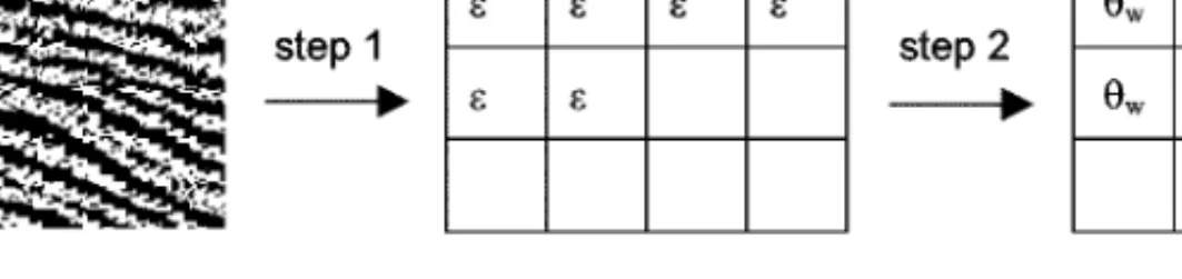
GPR is an imaging method that utilizes the transmission and reflection of high fre- quency (1 MHz to 1GHz) electromagnetic (EM) waves within the earth. Descrip- tions of the fundamental principles can be found in publications by Daniels et al (1988) and Davis & Annan (1989). A standard GPR survey is conducted by moving a transmitter and receiver antenna, separated by a fixed distance, along a survey line. The pair of antennas is moved to stations (measurement locations) with the spacing between stations determined by the survey objectives. At each station, a short pulse or “wavelet” of EM energy is sent into the earth by the trans- mitter antenna. The GPR wavelet contains a number of frequencies, but is usually referred to by the center frequency of the antennas, most typically 50, 100, 200, or 400 MHz. The reflected energy returned to the earth’s surface is recorded at the receiver antenna. The GPR image, an example of which is shown in Figure 1, is produced from a compilation of the station recordings.
The GPR image is a representation of the interaction between the transmitted EM energy and the spatial variation in the complex, frequency-dependent EM Annu. Rev. Earth Planet. Sci. 2001.29:229-255. Downloaded from www.annualreviews.org by University of Sydney on 04/10/13. For personal use only.
properties of the earth: the dielectric permittivityε, the electrical conductivityσ, and the magnetic permeabilityµ. The link between the radar image and these EM properties is best shown by considering the equations that describe the propagation of EM waves in the subsurface, as is done below. It is important to emphasize that the extent to which GPR can be successfully used for environmental applications is largely determined by the extent to which these EM properties are related to the presence or movement of a contaminant.
If we consider a single-frequency, linearly polarized, EM plane wave traveling in the z direction, we can derive, from Maxwell’s equations, the following expressions for the complex electric E and magnetic B field vectors,
E(z,t)=Eoe−αzei(ωt−βz)
and
B(z,t)=Boe−αzei(ωt−βz),
where Eo and Bo are the complex amplitudes,ω is angular frequency,αis the attenuation constant given by
α=ω rµε
2
"s 1+
µσ ωε
¶2
−1
#1/2
, andβis the phase parameter given by
β =ω rµε
2
"s 1+
µ σ ωε
¶2
+1
#1/2
.
The velocityvof the EM wave is given by v=ω
β.
In a field GPR survey, a measure of the velocity of the subsurface region is deter- mined by collecting data using a common midpoint geometry, where the distance between the transmitter and receiver antennas is increased gradually with each recording; this type of survey and the data analysis required to determine velocity is described in detail in Davis & Annan (1989). Information about the velocity of the subsurface can then be used to convert the recorded data, which show ampli- tude as a function of time, to a display of amplitude as a function of depth. For example, in the image in Figure 1, the maximum recorded arrival time of 140 ns corresponds to a depth of approximately 7 m.
There is a simplifying assumption commonly made in the interpretation of GPR data, that of “low-loss conditions,” which is expressed mathematically as the inequality σ/ωε <1. In general, this is a valid assumption given the high frequencies involved in GPR and the fact that the method cannot be used in regions where conductivity is too high; high values of σ result in a highly attenuative Annu. Rev. Earth Planet. Sci. 2001.29:229-255. Downloaded from www.annualreviews.org by University of Sydney on 04/10/13. For personal use only.
medium. An additional assumption generally made is thatµat all locations in the subsurface is equal to µ0, the magnetic permeability of free space (µ0 = 4 × 10⁻⁷henries/m). These assumptions result in the following simplified expressions for the velocity and attenuation constant,
v≈ 1
√µoε
and
α≈ σ 2
rµo
ε .
The above two expressions show that the dielectric permittivity controls velocity while the electrical conductivity has a large effect on attenuation. For this reason, GPR works well in regions composed of sands and gravels (which tend to be relatively resistive), but is of limited use in regions with electrically conductive clay. Clay content on the order of 5–10% can reduce the penetration depth of the radar to less than a meter (Walther et al 1986).
The amount of reflected energy seen in a GPR image is determined by the partitioning of the incident energy at any interface in the subsurface across which there is a change in EM properties. The amount of reflected energy can be expressed in terms of the reflection coefficient R, defined as the ratio of the complex amplitude of the reflected wave to that of the incident wave. For the simplified case of a normally incident EM wave with a smooth planar interface, where the incident wave’s electric field is polarized perpendicular to the plane of incidence (referred to as TE mode),
R=µ2k1−µ1k2 µ2k1+µ1k2
,
where subscripts 1 and 2 refer to the regions above and below the interface, and k is the wave number given by
k=β−iα.
Given the assumptions of low-loss and nonmagnetic media (µ = µ0), this sim- plifies to
R=
√ε1− √ε2
√ε1+ √ε2
.
Energy is thus returned to the surface from any depth at which there exists a discontinuity in the dielectric properties, and the amplitude of the returned energy is an indication of the level of contrast in the properties across the interface.
The expressions given above for the velocity and reflection coefficient show the way in which the dielectric structure of the subsurface affects what is seen in the GPR image. There are, however, numerous other factors such as the coupling of the antennas to the ground, the distribution of the radiated energy, and energy loss mechanisms that affect the radar image and can complicate interpretation of Annu. Rev. Earth Planet. Sci. 2001.29:229-255. Downloaded from www.annualreviews.org by University of Sydney on 04/10/13. For personal use only.
radar data. Some of these factors can be corrected for by using seismic processing and imaging methods (Fischer et al 1992a,b; Fisher et al 1996). This however requires the assumption that EM wave propagation is kinematically equivalent to the propagation of acoustic waves. One of the most important differences between the two is the strong frequency-dependence of many of the EM energy-loss mecha- nisms that causes a significant change in the frequency content of the GPR wavelet as it propagates in the subsurface (Turner 1994).
A way to gain insight into how dielectric properties, antenna characteristics, energy loss mechanisms, and other aspects of EM wave propagation determine what is seen in a radar image is to use forward modeling methods. Given a model of the subsurface in terms of dielectric properties, forward modeling algorithms can be used to produce the corresponding synthetic radar image (e.g. Powers 1995, 1997; Carcione 1996, 1998). Forward modeling is an active area of research as it allows us to better understand the fundamental physics governing the radar- imaging process and also has great practical value. Synthetic radar data are used to aid in interpretation and to predict how effective radar imaging will be for a given application and geological environment.
The use of radar images for near-surface applications can involve both qual- itative and quantitative interpretation of the recorded information. The methods currently used for processing and visualization of radar data make it possible to produce very high-quality radar images that can be used in a qualitative way to obtain information about the structure and stratigraphy of the subsurface and to locate regions of anomalous EM properties. In Figure 1, for example, is shown a GPR data set that was collected near Long Beach, Washington in a tectonically active coastal environment. The dipping surface, running from 10 m to 30 m and separating two regions of flat-lying reflections, has been interpreted as the uppermost boundary of an erosional scarp, related to earth- quake-induced subsidence (Meyers et al 1996). This “qualitative” interpre- tation of the radar data is aided by the high degree of clarity in the radar image; individual reflections are easily resolved and the image appears to be well focused.
For some applications we require more quantitative information about the phys- ical, chemical, and/or biological properties of regions of the subsurface. One way to approach this is to use the dielectric information contained in the radar image.
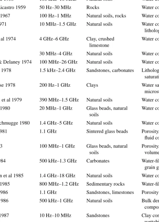
This can be described as a two-step process, as is shown schematically in Figure 2.
In step 1 we recover from the radar data a dielectric model. In step 2 we use rela- tionships between the dielectric permittivity and the subsurface property of interest to obtain a model of the spatial variation in that property (in this example water contentθw). The accuracy with which we can quantify subsurface properties is highly dependent upon our ability to obtain the dielectric model. Much more re- search is required before we will be able to use all of the reflected energy seen in a radar image in a quantitative way to extract an accurate, detailed, dielectric model of the subsurface.
The scale of measurement is an important issue that must be considered in using any method to characterize the subsurface; the role of scale and measurement Annu. Rev. Earth Planet. Sci. 2001.29:229-255. Downloaded from www.annualreviews.org by University of Sydney on 04/10/13. For personal use only.
Figure 2 Schematic illustration of the methodology used for the quantitative interpretation of a radar image to obtain a model of subsurface properties. Step 1 involves extracting a dielectric model from the radar data, where each “ε-block” is assigned a single dielectric permittivity (ε) value. Step 2 involves using the appropriate rock physics relationship to transformεin each block to the hydrogeologic property of interest, e.g. water contentθw.
in hydrogeologic studies was discussed by Beckie (1996). In data interpretation, there must be a recognition that the information obtained from a measurement is only valid over a certain range of scales, determined by a combination of the scale-dependent nature of the system under investigation and by the physics of the measurement method itself. One way to describe the scale of a radar measurement is in terms of resolution, which defines the smallest feature that can be seen or captured in the image. Both vertical and horizontal resolution are inversely pro- portional to the frequency of the radar measurement. Using the expressions given by Annan & Cosway (1994) to estimate the resolution in a saturated sand with 100 MHz antennas yields a vertical resolution of 1.3 m and a horizontal resolution of 2.4 m at a depth of 5 m. These approximate expressions are most likely to yield underestimates of the vertical resolution and overestimates of the horizontal resolution.
Another scale that is important in the use of radar images for applications in contaminant hydrology is the scale at which we can obtain dielectric information.
That is, if we were to recover from the radar image a dielectric model of the subsurface (step 1 in Figure 2), what is the scale at which we could assign values ofεto discrete regions of the subsurface? That is, what is the size of the “ε-blocks”
in Figure 2? This scale, which can be referred to as the support volume of the radar-based dielectric measurement, will be determined by both the resolution of the radar image and the specific algorithm used to obtain the dielectric model.
Given current methodologies, the best model that can be obtained will likely have linear dimensions on the order of several meters to tens of meters.
A GPR image is a representation of the dielectric properties of the subsurface.
When we use such an image for applications in contaminant hydrology, we are assuming that by imaging dielectric properties we are capturing information about the subsurface that is relevant for the detection of a contaminant or for predicting the fate and transport of the contaminant. In step 2 in Figure 2, which can be referred to as the “rock physics” step, we use an understanding of what controls the dielectric properties of geological materials to transform our dielectric model into a model Annu. Rev. Earth Planet. Sci. 2001.29:229-255. Downloaded from www.annualreviews.org by University of Sydney on 04/10/13. For personal use only.
of the subsurface properties of interest. This second step is critical: Dielectric properties do not govern contaminant transport directly (they govern EM wave propagation), but they are linked, through rock physics relationships, to the relevant material properties associated with the presence and transport of the contaminant.
DIELECTRIC PROPERTIES OF GEOLOGICAL MATERIALS
The dielectric properties of the subsurface are the primary control on both the amplitude and the arrival time of the received energy in a GPR survey. What we image in a GPR survey is thus largely determined by the variation in dielectric properties of the subsurface. If we can image a contaminant with GPR, it is because of a contrast in dielectric properties between the contaminated region and the background “clean” geological materials. If we can determine the hydrogeologic structure or heterogeneity of the subsurface it is because there is a link between the imaged dielectric properties and the hydrogeologic properties of interest. A critical question is, therefore, what controls the dielectric properties of materials in both clean and contaminated regions of the subsurface?
In general, the dielectric permittivity εand the electrical conductivityσ are complex, frequency-dependent parameters that describe the microscopic electro- magnetic properties of a material. The former accounts for mechanisms associated with charge polarization, whereas the latter accounts for mechanisms associated with charge transport. Following the sign convention adopted by Ward & Hohmann (1988), the conductivity and dielectric permittivity are defined as,
σ (ω)=σ0(ω)+iσ00(ω) and
ε(ω)=ε0(ω)+iε00(ω),
where ωis angular frequency, ε0(ω) is the polarization term, ε00(ω) represents energy loss due to polarization lag,σ0(ω) refers to ohmic conduction, andσ00(ω) is a faradaic diffusion loss. A detailed discussion of the mechanisms governing these four parameters in Earth materials can be found in Powers (1997) and Olhoeft (1998).
The total response of a material to an oscillating electric field will incorporate all of these mechanisms and can be described either in terms of a total complex permittivity or total complex conductivity. For the purposes of discussing the role of dielectric properties in radar, it is preferable to use the total complex permittivity εT(ω) given by
εT(ω)=[ε0(ω)−iε00(ω)]− i
ω[σ0(ω)+iσ00(ω)].
When the right-hand side of this equation is rearranged, we can form a real part representing the ability of the material to store energy through polarization and Annu. Rev. Earth Planet. Sci. 2001.29:229-255. Downloaded from www.annualreviews.org by University of Sydney on 04/10/13. For personal use only.
an imaginary part representing the ability of the material to transport charge. The resulting real-valued, “effective” permittivity and conductivity are:
εef(ω)=Re{εT(ω)} =ε0(ω)+σ00ω ω and
σef(ω)= −ωIm{εT(ω)} =σ0(ω)+ωε00(ω).
It is commonly assumed that σ00(ω)=0 and thatσ0(ω)=σDC, the frequency- independent direct current (D.C.) conductivity of the material. For notational simplicity, the (ω) designation will be dropped for the remainder of this review.
The quantity commonly referred to as the dielectric constant,κ, is defined as κ =εef
εo
,
whereεois the permittivity of free space. The expressions given earlier for the EM wave velocity and reflection coefficient in a low-loss nonmagnetic medium can be written in terms ofκas follows:
v= c
√κ and
R=
√κ1− √κ2
√κ1+ √κ2
,
where c (the speed of light in free space) is equal to 3×10⁸m/s.
The dielectric constants of many of the individual components encountered in near-surface studies are well known: For pure waterκ = 80; for pure quartzκ = 4.5; for airκ =1; other solid minerals have values ofκranging approximately from 5 to 10. The dielectric properties of a number of contaminants have been measured (along with other useful properties) and are compiled in Lucius et al (1992).
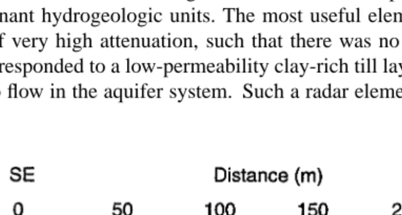
There have also been numerous laboratory studies of the dielectric properties of various rocks, sediments, and solids, to determine how κ of the total system (solids and fluids) is affected by frequency of measurement and various material properties such as composition, porosity, water content, and microgeometry. Some of these laboratory studies, relevant to environmental applications of GPR where measurements were made in the frequency range of 1Mz to 1GHz, are summarized in Table 1 (which is a modified version of Table 1 in Knoll 1996).
The laboratory studies and complementary theoretical studies provide a foun- dation for understanding the controls on the dielectric properties of near-surface materials. Based on this body of work we can describe the dielectric constant of any multicomponent geological material as being determined by:
1. the volume fractions and dielectric constants of the individual components, 2. the geometrical arrangement or distribution of the components,
Annu. Rev. Earth Planet. Sci. 2001.29:229-255. Downloaded from www.annualreviews.org by University of Sydney on 04/10/13. For personal use only.
TABLE 1 Experimental investigations of the dielectric properties of geological materials Reference Frequency Range Material Physical Properties Studied
Smith-Rose 1933 100 kHz–10 MHz Natural soils Water content Keller & Licastro 1959 50 Hz–30 MHz Rocks Water content Scott et al 1967 100 Hz–1 MHz Natural soils, rocks Water content
Lundien 1971 10 MHz–1.5 GHz Natural soils Water content, bulk density, lithology
Birchak et al 1974 4 GHz–6 GHz Clay, crushed Water content limestone
Hipp 1974 30 MHz–4 GHz Natural soils Water content, bulk density Hoekstra & Delaney 1974 100 MHz–26 GHz Natural soils Water content
Poley et al 1978 1.5 kHz–2.4 GHz Sandstones, carbonates Lithology, porosity, water saturation
Hall & Rose 1978 200 Hz–1 GHz Clays Water saturation, clay microstructure Okrasinski et al 1979 390 MHz–1.5 GHz Natural soils Water content, porosity Topp et al 1980 20 MHz–1 GHz Glass beads, natural Water content
soils
Wang & Schmugge 1980 1.4 GHz–5 GHz Natural soils Water content, clay content Sen et al 1981 1.1 GHz Sintered glass beads Porosity, geometry, pore
fluid content
Lange 1983 100 MHz–1 GHz Glass beads, natural Porosity, surface area/pore
soils volume, saturation
Kenyon 1984 500 kHz–1.3 GHz Carbonates Water-filled porosity, grain geometry
Hallikainen et al 1985 1.4 GHz–18 GHz Natural soils Water content, clay content Shen et al 1985 800 MHz–1.2 GHz Sedimentary rocks Water-filled porosity Sherman 1986 1.1 GHz Sandstones, limestones Porosity
Kutrubes 1986 500 kHz–1 GHz Natural soils Bulk density, fluid composition Garrouch 1987 10 Hz–10 MHz Sandstones Clay content, salinity,
wettability, stress Knight & Nur 1987a 60 kHz–4 MHz Sandstones Water saturation, surface
area/pore volume Knight & Nur 1987b 10 kHz–4 MHz Sandstones Pore-scale fluid distribution Olhoeft 1987 0.001 Hz–1 GHz Sand-clay mixtures Porosity, water saturation,
clay content Taherian et al 1990 10 MHz–1.3 GHz Sandstones, carbonates —
Knoll & Knight 1994 100 kHz–10 MHz Sand-clay mixtures Clay content, porosity Knight & Abad 1995 1 MHz Sandstones Solid/fluid interactions Knoll et al 1995 100 kHz–10 MHz Sand-clay mixtures Permeability Annu. Rev. Earth Planet. Sci. 2001.29:229-255. Downloaded from www.annualreviews.org by University of Sydney on 04/10/13. For personal use only.
3. the physical and/or chemical interactions between components.
The role of these parameters is best shown by considering the various methods that can be used to model the total dielectric constant. These methods include volu- metric averaging models, empirical relationships, and effective medium theories.
Volumetric averaging models are semi-empirical and provide a means of esti- mating the average or total dielectric constant of a sampled volume that is made up of a number of individual components of known dielectric constants and volume fractions. For example, in the vadose zone of the earth, above the water table, the dielectric constant of a sampled volume would be related to the dielectric constants of the solid component, the water, and the air. These models take the general form,
κavgn =6θκin,
where κavg is the average dielectric constant of the sampled volume, θiis the volume fraction of a component,κiis the dielectric constant of that component, and n is a constant to account for the geometrical arrangement of the components (Lichtenecker & Rother 1931). The two endmembers, n = 1 and n = −1 corres- pond to the cases where all the components are aligned perpendicular and parallel to the propagating EM wave. Mathematically we can describe the true geometry of a material as lying between these two bounds.
Despite the apparent simplicity of such an approach, remarkably good agree- ment has been found in modeling the dielectric properties of geological materials in the radar frequency range with the above equation with n =1/2. This is known as the complex refractive index model (CRIM) (Wharton et al 1980). This sim- ple expression predicts what has been found to be the dominant control onκ of near-surface materials—the water content—due largely to the contrast betweenκ of water (80) andκ of the other components (∼1–10). Note, however, the num- ber of studies in Table 1 with a focus on understanding the relationship between dielectric properties and water content. Clearly if CRIM were a completely ac- curate model, these studies would not be needed. There are other factors such as the microgeometry of the solid and fluid phases, solid/fluid interactions, and the frequency of the measurement that are not accounted for in CRIM. Despite these limitations, CRIM is commonly used to assess the potential usefulness of GPR for contaminant detection and to derive water content or saturation from field measurements of dielectric constant.
A second approach to modeling dielectric data is the use of empirical relation- ships. The relationship introduced by Topp et al (1980) is widely used to model the strong dependence of the measured dielectric constant on water contentθw:
κavg=3.03+9.30(θw)+146.00(θw)2−76.70(θw)3.
This equation was determined from regression analysis of data obtained for four different soils with varying water content and with clay content ranging from 9 to 66% by weight. The Topp equation has become one of the standard methods for extracting water content from dielectric measurements. While the Annu. Rev. Earth Planet. Sci. 2001.29:229-255. Downloaded from www.annualreviews.org by University of Sydney on 04/10/13. For personal use only.
advantage of using this equation is that no information is required about the sampled material, the obvious disadvantage is its empirical nature and therefore limited expected accuracy especially in areas where the materials differ from those used in developing the relationship.
A more rigorous approach to modeling the dielectric response of a material is the use of effective medium theories. A useful review of the development of the various classes of these theories is given by Landauer (1978). The use of an effective medium theory (EMT) allows one to explicitly incorporate effects such as the geometry of the components in predicting dielectric properties. One example of an EMT that has been applied to geological materials is the Hanai- Bruggeman-Sen model (Bruggeman 1935, Hanai 1961, Sen et al 1981). This model, which was developed to model the dielectric properties of a porous solid saturated with a single fluid phase, accounts for the permittivities of the solid and fluid, the volume fractions of the two components through the porosity term ø, and the microgeometry through a “depolarization factor,” which describes the aspect ratio of the grains.
It has been determined, through laboratory studies and theoretical modeling, thatκ depends on both the water-filled porosity of a geological material and the microgeometry of the solid phase. The fact that these are also key parameters in determining the permeability of a material raises the intriguing possibility that radar-based dielectric measurements can provide information about this hydroge- ologic property. Figure 3 shows the results from a laboratory study of sand/clay mixtures (Knoll et al 1995) where both κ and the permeability of the samples were measured. The experimental data show thatκof the dry samples is relatively
Figure 3 Laboratory measurements of the dielectric constant of sand-clay mixtures versus the permeability. Dielectric measurements were made at a frequency of 1 MHz on a set of water-saturated samples (solid symbols) and dry samples (open symbols). The dotted lines show the relationships predicted using the Kozeny-Carmen equation. Adapted from Knoll et al (1995).
Annu. Rev. Earth Planet. Sci. 2001.29:229-255. Downloaded from www.annualreviews.org by University of Sydney on 04/10/13. For personal use only.
insensitive to permeability. In the saturated samples the observed dependence of κ on permeability is well modeled using the Kozeny-Carmen equation (Kozeny 1927, Carmen 1956) and can be explained by the fact that bothκand permeability are governed primarily by the volume fraction of the pore space (porosity) and the microgeometry of the pore space, as quantified by the specific surface area of the material. (The v-shaped curve is due to the porosity variation that occurs as the sample composition is varied from 100% clay to 100% sand.)
While we have a reasonably complete understanding of the dielectric properties of “clean” materials, there is a surprising lack of laboratory and theoretical studies of materials containing contaminants. In laboratory measurements of sands sat- urated with benzene and methane, the Hanai-Bruggeman-Sen model was found to accurately predictκ of the sand saturated with a single fluid (Kutrubes 1986), but could not predictκ of a sand containing two fluids. Clearly, there are factors associated with the presence of two fluids that are not included in this model. Lab- oratory studies have shown that both the pore-scale geometry of the fluid phases and solid-fluid interaction can affectκ of a fluid-saturated sample (Knight & Nur 1987b, Knight & Endres 1990, Knight & Abad 1995, Garrouch 1987). A study by Endres & Redman (1996), which considers the dielectric response of a porous material saturated with an organic contaminant and water, illustrates the poten- tial significance of these effects in determining measured dielectric properties in contaminated materials. Clearly dielectric constants, volume fractions, the micro- geometry of solids and fluids, and solid/fluid interactions must all be considered when interpreting or predicting the dielectric properties of clean and contaminated geological materials.
Over the past 10–15 years, a good understanding has developed of the dielectric properties of geological materials based on laboratory and theoretical studies. It is important to note however, that most of this work has involved laboratory studies with small, homogeneous samples, and the development of corresponding theo- ries, valid for small, homogeneous systems. As a result, all of the relationships that are currently used to relate the radar-based dielectric measurements to param- eters of interest such as fluid content (of water, air, or contaminant), porosity, or permeability are of the forms described above, and have one key limitation: All of them are valid only if the sampled volume is homogeneous. As we attempt to ex- tract detailed information about the properties of the subsurface from radar-based dielectric measurements, we face the challenge of upscaling the rock physics re- lationships and extending our understanding of dielectric properties of geological materials to encompass the heterogeneity of natural systems.
CAN WE DETECT CONTAMINANTS WITH RADAR DATA?
The most obvious use of GPR for applications in contaminant hydrology is for the direct detection of a contaminant. This review of contaminant detection with GPR will address the specific issue of detection of immiscible liquid-phase or- ganics, which has been a major focus within the geophysical community. In the Annu. Rev. Earth Planet. Sci. 2001.29:229-255. Downloaded from www.annualreviews.org by University of Sydney on 04/10/13. For personal use only.
United States, this is largely driven by the fact that most of the contamination, at the many thousands of hazardous waste sites, is from organic compounds such as trichloroethylene, gasoline, and other solvents and fuels (Walther et al 1986).
The ability of GPR to detect a contaminant requires that the presence of the contaminant perturbs the dielectric properties of the subsurface sufficiently to result in a detectable change with the GPR measurement. As discussed above, the dielectric properties of a multicomponent material are determined, to a first approximation, by the volume fractions and dielectric constants of the individual components. The dielectric constants of the top 10 organic contaminants, listed with respect to frequency of occurrence range from approximately 2 to 10 (Lucius et al 1992). For example, the first three on this list are trichloroethylene (TCE), κ=3.42 (measured at 10◦C); dichloromethaneκ =8.93 (measured at 25◦C); and tetrachloroethylene or perchloroethylene (PCE):κ =2.28 (measured at 25◦C).
Given the contrast between these values of κ for an organic contaminant and that of water (κ =80), it is clear that if a contaminant displaces water in a region of the subsurface, there will be a distinct change in the dielectric constant of that region.
The first well-known controlled field experiment conducted specifically to as- sess the use of GPR for the detection of organic contaminants was the work per- formed in 1991 at the Borden field site by the University of Waterloo and described in a series of publications (Greenhouse et al 1993, Brewster & Annan 1994, Sander 1994, Brewster et al 1995). A total of 770 L of PCE was introduced through an injection well into a sand-filled cell, 9 m×9 m×3 m deep. Injection occurred over a period of 70 hours with GPR data collected at regular intervals up to 340 hours after the start of the spill. The GPR images of PCE, which is den- ser than water, sinking through a water-saturated sand provided convincing evi- dence that monitoring of contaminant movement with radar data is in fact possible.
A series of 500 MHz radar images from this study are reproduced in Figure 4.
In the top image is the starting condition. Within the homogeneous sand there are reflections interpreted as corresponding to subtle changes in porosity. Subse- quent images show the development of high amplitude reflections, which cor- respond to the migration of the PCE. The presence of the contaminant, with κ = 2.3 displacing water with κ =80, created a zone with a relatively high reflection coefficient. Using CRIM to estimate values ofκ, reflection coefficients were predicted of R = 0 with no PCE present, R = 0.05 with 15% of the pore volume filled with PCE, R = 0.11 with 30% of the pore volume filled with PCE, and R = 0.49 for the case of 100% saturation with PCE (Greenhouse et al 1993).
The data are interpreted to show a combination of ponding, lateral spreading, and downward movement of the contaminant. It is interesting to note that, even in this controlled experiment in a cell packed with homogeneous sand, the contaminant follows a complex path.
This experiment not only illustrated the potential use of GPR to detect contami- nants when location and clean-up is the objective, but also illustrated the significant value of GPR as an imaging method for the purpose of studying the dynamics of Annu. Rev. Earth Planet. Sci. 2001.29:229-255. Downloaded from www.annualreviews.org by University of Sydney on 04/10/13. For personal use only.
contaminant migration in a large-scale experiment. Rather than an instrumented laboratory-scale experiment to determine the controls on contaminant movement, GPR can be used as a means of imaging and thereby studying transport processes on a much larger scale. The resolution of the radar imaging is such that valuable information can be obtained about the effects on transport of spatial heterogeneity within natural geologic systems.
The radar images from the Borden experiment should be taken as examples of the best images of a contaminant that could be obtained in a natural setting using currently available technologies. Because of the homogeneity of the sand at Borden, the largest reflection coefficients were associated with the interface between the contaminated and water-saturated regions. In general, the hetero- geneity of natural geologic systems will result in a myriad of reflections with a wide range of reflection coefficients; the challenge then becomes distinguish- ing between a reflection caused by a contaminant and a reflection caused by changes in the geological materials such as changes in porosity or lithology. In the Borden experiment, the availability of an image of the starting condition at the site removed any ambiguity as to the location of the contaminant in the radar images.
While it is rare to have a radar image of a site prior to contamination, the imaging of changes, or subtractive imaging (where two images acquired at different times are subtracted to show the change) is a very effective way to distinguish reflections associated with the contaminant from reflections associated with the background geology: The locations of the former will change with time. Based on the idea of subtractive imaging, there is considerable interest in using GPR as a means of monitoring contaminant movement or contaminant removal during remediation.
Not surprisingly, radar images from field studies tend to show highly vari- able responses to the presence of a contaminant. As reviewed by Grumman &
Daniels (1995), there are a number of effects that the presence of an organic contaminant can be expected to have on radar data; given in this reference are examples of field or modeling studies. Many studies report the appearance of an “anomalous region” in the radar image where the pattern or amplitude of the reflections is altered in the contaminated area. In many cases, the fundamental cause is the fact that a contaminant with a lowκ is replacing water with a highκ, which leads to changes in the amplitude of the reflections, and changes in the EM velocity.
A fascinating area of research (which can perhaps be called “biogeophysics”) has been recently triggered by attempts to better understand the relationship be- tween the presence of a contaminant and what is seen in the radar image. Over the past 10–12 years, there have been recurring descriptions in the literature of a region with a “washed out” or muted appearance in the radar data corresponding to, or overlying, a region of known hydrocarbon contamination (Olhoeft 1986; Benson 1995; Daniels et al 1992, 1995; Maxwell & Schmok 1995; Sauck et al 1998; King 2000). Although various explanations have been proposed for the cause of the apparent increased attenuation in the radar data, there is still no clear consensus as to what is responsible for this observation. A novel idea, described in a recent series of papers (Sauck et al 1998, Atekwana et al 2000, Lucius 2000, Sauck 2000, Annu. Rev. Earth Planet. Sci. 2001.29:229-255. Downloaded from www.annualreviews.org by University of Sydney on 04/10/13. For personal use only.
Werkema et al 2000), is that bacterial activity leads to an increase in the electrical conductivity of the region adjacent to the contaminant, thus increasing the attenu- ation of the radar signal. (As seen in the equation for EM attenuation,αis directly proportional to the electrical conductivity.)
Very briefly, the proposed mechanism starts with the bacterial breakdown of the hydrocarbon. This process produces organic or carbonic acids, which cause mineral dissolution. The mineral dissolution increases the ionic content of the pore fluid, resulting in an increase in the electrical conductivity (and EM attenu- ation) of the sediments. The net result is that the hydrocarbon-contaminated sed- iments, typically measured in the laboratory to be electrically resistive relative to water-saturated sediments, become electrically conductive because of the natural biodegradation of the contaminant. The presence of the hydrocarbon in the sub- surface therefore corresponds to a conductive, attenuative region in the radar data.
Recent work at a field site provides strong support for this model of temporal changes in the electrical properties of a contaminated region. A strong correlation was found between the location of high conductivity zones, the presence of the hydrocarbon contaminant, and order of magnitude increases in bacterial counts, in particular “oil degraders” (Werkema et al 2000). This ongoing research, which addresses the role of bacterial activity in defining in situ electrical properties, has served as a wake-up call to the rock physics community. Although we have tended to carefully control physical and chemical conditions during laboratory measurements on near-surface materials, a control of biological conditions, such as the level of bacterial activity, has been completely neglected.
In some cases anomalous regions as described above can be readily identified in radar images and used as a means of locating a contaminated area. In general, however, the use of GPR as a definitive method for locating and quantifying the amount of the contaminant is limited by a lack of understanding of the effect of the contaminant on the dielectric properties and the resulting radar image. The further development of GPR as a means of direct detection of subsurface contaminants requires a combination of well-characterized field studies and the complementary laboratory and theoretical work. It is impossible to accurately predict the dielectric response of contaminants without laboratory-based observations of porous fluid- saturated materials under conditions—physical, chemical, and biological—that are representative of in situ conditions.
OBTAINING A HYDROGEOLOGIC MODEL OF THE SUBSURFACE
Once the location of subsurface contamination has been identified, using either direct sampling or geophysical methods, decisions must be made about the short- term and long-term strategies for dealing with the contaminated region. The vari- ous options can include physically removing contaminated materials, treating the contaminant in situ, physically isolating the contaminant through the use of im- permeable barriers, and electing to do nothing. (The “do nothing” option does Annu. Rev. Earth Planet. Sci. 2001.29:229-255. Downloaded from www.annualreviews.org by University of Sydney on 04/10/13. For personal use only.
not necessarily imply no positive change in the state of the contaminated region as natural processes of biological breakdown of the contaminant, referred to as bioremediation or natural attenuation, can occur.) Assessment of these various options generally involves the development of a model of the subsurface that can be used to predict the fate and transport of the contaminant.
Given the large volume of data required to develop an accurate model of the subsurface, and the limitations of direct sampling, the use of geophysical methods can contribute significantly to the challenge of obtaining information about the subsurface. Using radar data to develop a model of the subsurface can be described as involving two stages of characterization. The first is to obtain a model of the three-dimensional architecture of the subsurface region of interest. This involves mapping out geologic units at a scale of meters to 10’s or 100’s of meters and identifying any large-scale features, such as the water table, faults, or fractures, that are critical to the contaminant transport model. In order to use such a model to predict transport, hydrogeologic properties such as porosity, water content, and permeability need to be determined. The second stage in characterization is to use the radar data to assist in obtaining estimates of these properties that can then be assigned to regions within the large-scale model.
Radar Imaging of the Large-Scale Architecture
The extent to which radar images can be used as a basis for the development of hydrogeologic models is clearly dependent upon the quality of the radar image. In systems dominated by materials with low electrical conductivity, it is possible to obtain radar images of very high quality. Most of the published examples of GPR data to date are from sedimentary environments; this is due to the fact that GPR has been widely used in the past 10–15 years to study both modern and ancient sedimentary systems. As examples, excellent radar images of fluvial deposits can be seen in the recent publication by Vandenberghe & van Overmeeren (1999).
Let us consider the GPR image shown in Figure 1. If our objective was to develop a hydrogeologic model to predict contaminant movement through the imaged region, we could build our model using, as a starting point, the large-scale architecture seen in the GPR image. This assumes that the large-scale architecture seen in the radar image is also the large-scale architecture relevant to the movement of fluids in the subsurface. To construct the model, we could define boundaries within the radar image based on the location of the dominant reflections and divide the image into regions of similar character or appearance. This approach has been formalized into a concept referred to as radar facies analysis, first applied in the early 1990s in the work of Baker (1991), Beres & Haeni (1991), and Jol & Smith (1991).
Radar facies analysis involves dividing the radar image into regions that have a common appearance, referred to as radar facies units. A radar facies unit is defined by Baker (1991) as “groups of radar reflections whose parameters (configuration, amplitude, continuity, frequency, interval velocity, attenuation, dispersion) differ from adjacent groups. Radar facies are distinguished by the types of reflection Annu. Rev. Earth Planet. Sci. 2001.29:229-255. Downloaded from www.annualreviews.org by University of Sydney on 04/10/13. For personal use only.
boundaries, configuration of the reflection pattern within the unit and the external form or shape of the unit.” Shown in Figure 5 is an example of a radar profile, from the active lacustrine Sandy Point spit in northeastern Alberta, where the radar facies concept was used in interpretation (Smith & Jol 1992). The bottom 2 m of the radar profile, made up of continuous, horizontal reflections is defined as one radar facies unit that has been interpreted to represent the lake bed. The overlying section of inclined reflections, a second radar facies unit, is interpreted to represent the middle to lower shoreface. The top 3 m of the radar profile, the third radar facies unit, contains horizontal to slightly inclined reflections, which are interpreted to represent beach foreshore and upper shoreface deposits.
The concept of radar facies analysis has been used extensively in some areas to aid in the development of hydrogeologic models of the subsurface. A 10-year effort, involving 30 km of data collection, has been undertaken in the Netherlands to compile the characteristic radar signatures of most of the sedimentary environments suitable for GPR surveys (van Overmeeren 1996, 1998). The imaged environments include glacial, aeolian, fluvial, lacustrine, and marine. Radar data from new areas can be readily interpreted and incorporated into hydrogeologic models by reference to the GPR “calibration” images.
A similar concept of using “radar architectural elements” was applied to a study of the Brookswood aquifer in southwestern British Columbia (Rea & Knight 1995, 2000). The Brookswood is an unconfined aquifer, where concern about surface contamination meant that a detailed model of the lateral continuity of the aquifer units was needed. Over 12 km of radar data were divided into radar elements, and information from drillers’ logs was used to relate specific radar elements to the dominant hydrogeologic units. The most useful element was one defined as a zone of very high attenuation, such that there was no radar response. This element corresponded to a low-permeability clay-rich till layer, which serves as a boundary to flow in the aquifer system. Such a radar element is a key feature of
Figure 5 Ground penetrating radar (GPR) profile collected over the active Sandy Point spit in northeastern Alberta. Adapted from Smith & Jol (1992).
Annu. Rev. Earth Planet. Sci. 2001.29:229-255. Downloaded from www.annualreviews.org by University of Sydney on 04/10/13. For personal use only.
model development as it can be used to locate barriers to contaminant movement within the aquifer system.
In addition to using radar images to locate stratigraphic boundaries, radar data can also be used to locate some of the other important large-scale features re- quired in a hydrogeologic model. GPR has been successfully used in a number of field studies to delineate the boundary between the vadose zone and the saturated zone (Knoll et al 1991, van Overmeeren 1994, Iivari & Doolittle 1994, Doolittle et al 2000, Endres et al 2000), and has been used to detect faults and fractures in crystalline rocks (Davis & Annan 1989, Grasmuck & Green 1996). An example of the former is shown in Figure 6. Imaged in this data set (described in detail in Knoll et al 1991) are the dipping sands and gravels of the aquifer unit at the US Geological Survey Hydrology Research site on Cape Cod; the dominant reflection at approximately 10 ft is the top of the saturated zone. When this radar image is displayed in such a way as to preserve only the highest amplitude reflections (Figure 7) the top of the saturated zone can be clearly seen because of the large value of the reflection coefficient at the interface between the saturated and unsaturated regions.
In using a radar image as the basis for a hydrogeologic model, we are assuming that there is a relationship between the features that are imaged in the radar data and the structure and properties of the subsurface that control fluid movement.
Given that reflections in the radar image correspond to interfaces across which there is a change inκ, we can expect the presence of reflections and the magnitude of R (the reflection coefficient) to be closely related to any property or process that controls the location of water. In the water-saturated region of the subsurface, this provides a link between the radar image and water-filled porosity, an important hydrogeologic property.
A change in water content is clearly not the only cause of reflections in a radar image. In a very informative exercise, Baker (1991) used the Hanai-Bruggeman- Sen effective medium theory to predict dielectric properties and reflection coeffi- cients that would correspond to sedimentological interfaces within a coastal beach environment. The predicted reflection coefficient varied from 0.013 because of a 5% change in porosity in a dry sand, to 0.43 at lithologic boundary. These results show that even minor changes in physical properties may be detectable with radar, but also illustrate the inherent nonuniqueness in making a geological interpretation of a radar section.
Ideally, at any site where a hydrogeologic model is constructed with the use of radar data, there will be a way to “calibrate” the radar image or elements and deter- mine the link to the hydrogeology. In some cases, such as in the study conducted by Rea & Knight (2000), the radar image can be calibrated with information from wells. In other cases, a useful approach is to conduct cliff face experiments, where a radar unit can be moved along the top of the cliff and the radar image compared directly to the exposed vertical section. This is an excellent way to better under- stand what sedimentary features can be seen in radar data. A third approach is the use of forward modeling, where the geologic section is represented as a di- electric section and used to produce a synthetic radar image. Forward modeling Annu. Rev. Earth Planet. Sci. 2001.29:229-255. Downloaded from www.annualreviews.org by University of Sydney on 04/10/13. For personal use only.
is a very useful way to develop a fundamental understanding of the link between what is actually present in the subsurface and what will be captured in the radar image.
Given the current capabilities for the collection, processing, and visualization of radar data, high quality images can be obtained from a wide range of geologic environments. These images can be used as the basis for the development of hydrogeologic models. Although this requires an understanding of the relationship between the imaged dielectric structure and the required hydrogeologic structure, a radar image will often provide the best available constraint on the large-scale architecture of the subsurface.
Estimates of Subsurface Properties
Once a model of the large-scale structure has been obtained, the next step is that of assigning hydrogeologic properties to the various modeled units. In order to predict the long-term movement of a contaminant through an area, information is required about hydrogeologic properties such as water content, porosity, and permeability. Radar data can potentially be used for this purpose by extracting a three-dimensional dielectric model from the data and then using determined relationships between dielectric properties and the hydrogeologic properties of interest to transform the dielectric model into a hydrogeologic model. This was shown schematically in Figure 2, where various regions in the subsurface are assigned values ofε, and thatε-model is converted to the property of interest: in that case moisture content.
The first step in this approach is obtaining the three-dimensional model of the permittivity. Ideally all of the information in a standard radar profile would be used to determineεat all depths for all recorded data. Although this would give us a dielectric model with submeter scale resolution, this is far beyond current modeling capabilities. An alternate approach is to use the common midpoint geometry (typically only used at a few locations in a standard GPR survey) to determine the EM velocity at many locations. The velocity model, which assigns values of EM velocity to discrete volumes in the subsurface, can then be used to obtain a dielectric model (using the relationship between v and ε), and the appropriate relationship used to estimate the property of interest in the discrete volumes. An example of this approach is given in the study by Greaves et al (1996), the result being a two-dimensional model of EM velocity resolved at the scale of approximately 10 m ×10 m. Using the Topp equation, a two-dimensional model of water content in the subsurface was obtained.
One of the critical issues in the link between the ε-model of the subsurface and the hydrogeologic model is the heterogeneity of the system at the scale of the dielectric measurement. With the current modes of data acquisition and analysis, the size of the volume at whichεis determined (i.e. the size of theε-blocks in Figure 2) is on the order of meters to tens of meters. At this scale, it is very likely that each of the ε-blocks represents a system that is heterogeneous at smaller scales. Yet the relationships that are used in step 2 in Figure 2, to obtain estimates Annu. Rev. Earth Planet. Sci. 2001.29:229-255. Downloaded from www.annualreviews.org by University of Sydney on 04/10/13. For personal use only.
of subsurface properties, are most commonly of the form that assume that each ε-block can be treated as a homogeneous system. Simple models of geologic systems have shown that neglecting the heterogeneity can lead to significant errors in estimates of water content (Chan & Knight 1999). What is required is a means of quantifying the heterogeneity that exists within the sampled regions if radar- based dielectric measurements are to be used to provide accurate estimates of hydrogeologic properties.
The need to quantify spatial heterogeneity introduces another way in which radar data can be used in estimating hydrogeologic properties. This can be de- scribed as an image-based approach where, rather than assigning dielectric and hydrogeologic properties to specific volumes in the subsurface, we use all of the submeter scale information that can be seen in the radar image to quantify the spatial variability in the properties. A number of researchers (Olhoeft 1991, Young 1996, Tereschuk & Young 1998, Rea & Knight 1998) have found very encouraging results suggesting that the spatial variability or the correlation structure seen in radar images is representative of the spatial variability of the subsurface.
Geostatistical analysis of radar data has been found to be an effective way of quantifying the correlation structure of radar images from glaciofluvial, barrier spit, and deltaic environments (Rea & Knight 1998, Tercier et al 2000). The exper- imental semivariogram is used to describe the way in which the difference between data values is related to their separation distance and is described by the following equation (Deutsch & Journel 1992):
γ (h)= 1 2 N(h)
N(h)
X
i=1
[z(xi+ h)−z(xi)]2,
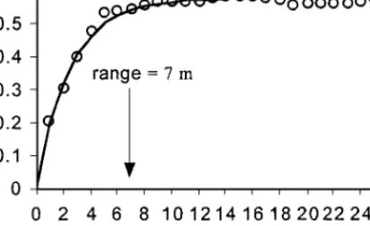
where h is the lag, or separation vector, between two data points, z(x+h) and z(x); and N is the number of data pairs used in each summation. In the analysis of radar images, the data values are the amplitudes of the reflected energy. Shown in Figure 8 is the semivariogram (from Tercier et al 2000) that was obtained from analysis of the middle radar facies unit in the GPR image in Figure 4. Two-dim- ensional geostatistical analysis of the image indicated that the direction of maximum correlation is along a line plunging 2◦ southeast; the semivariogram in Figure 8 was obtained using a lag vector oriented in that direction. This is a text-book example of a variogram and illustrates how well this approach works as a means of quantifying the spatial variability seen in a radar image. Modeling of the experimental variogam gave a correlation length of 7 m for this image.
In many environmental applications there will exist some knowledge of hy- drogeologic properties determined at specific locations (e.g. from drilling and direct sampling). The challenge is interpolating between what are usually sparsely sampled data points to obtain a higher resolution model of subsurface properties.
If what is seen in a radar image can be taken as representative of the spatial vari- ability of the subsurface materials, analysis of radar images could be an invaluable aid in generating accurate subsurface models without the need for extensive direct sampling. The magnitude of hydrogeologic properties could be determined at a Annu. Rev. Earth Planet. Sci. 2001.29:229-255. Downloaded from www.annualreviews.org by University of Sydney on 04/10/13. For personal use only.
Figure 8 Semivariogram analysis of the middle region in Figure 5. The data points are the circles; the model of the semivariogram is the solid line. The data are modeled using an exponential model with a range of 7 m. Adapted from Tercier et al (2000).
few locations and the heteogeneity, as quantified from the GPR image, used to generate the detailed model. Although research on this topic is ongoing, this might be one way in which the detail seen in the radar image can be used along with other sources of information to constrain hydrogeologic models.
CONCLUSIONS
There is a tremendous need for the development of noninvasive technologies that can be used to obtain quantitative information about contaminated regions of the subsurface. This need arises because of recognized limitations in the traditional methods of subsurface characterization. The ultimate goal in using GPR for ap- plications in contaminant hydrology can be described as taking an image, such as that shown in Figure 1, and transforming it into a quantitative image of the relevant physical, chemical, and biological properties of the subsurface. While it is possible at present to extract useful information about large-scale structure, we are still limited in our ability to obtain accurate, quantitative information about the subsurface properties of interest at the required scale.
There is one fundamental problem that we face in attempting to interpret GPR data: The information provided by a GPR measurement is far too limited given the spatial complexity of the subsurface. This problem is not unique to GPR data. It is a general challenge in the interpretation of subsurface measurements—geophysical and other—and highlights the need to take a multifaceted approach to charac- terization and to combine various sources of data. Significant advances in the use of geophysical data for subsurface characterization are likely to be made if the geophysical data, rather than being acquired and interpreted in isolation, are Annu. Rev. Earth Planet. Sci. 2001.29:229-255. Downloaded from www.annualreviews.org by University of Sydney on 04/10/13. For personal use only.
closely integrated with other forms of subsurface measurement. Some researchers have proposed specific methodologies that can be used to integrate measurements obtained from radar data with those obtained from standard hydrogeologic test- ing (Poeter et al 1997; Hubbard et al 1997, 1999; Chen et al 1999; Hubbard &
Rubin 2000). A recent example is the study by Chen et al (1999) in which surface radar data were used along with tomographic seismic and radar data to improve estimates of permeability at the Department of Energy Oyster Site in Virginia.
GPR is a high resolution geophysical technique that can provide remarkable images of the subsurface of the earth. Contained in these images is a wealth of information; extracting this information is a focus of ongoing research. A GPR image represents the interaction between EM waves and the dielectric prop- erties of the earth. It is deciphering the link between the resulting radar image and the subsurface properties and processes of interest that underlies the future usefulness of GPR for applications in contaminant hydrology.
ACKNOWLEDGMENTS
I would like to acknowledge the many people at the University of British Columbia with whom I have shared an interest in ground penetrating radar. Much of this paper is the result of discussions and time spent with all of you. In particular I wish to thank Mike Knoll, for stimulating my interest in GPR and initiating this area of research at UBC; Ana Abad, for her assistance in the laboratory;
Jane Rea, for the collection of over 20 km of radar data; James Irving, for field work in the heat of Texas and the dust storms of Hanford; Tony Endres, for his insights into the theoretical modeling of dielectric properties; Christina Chan, for her measurements and modeling of EM wave velocities; Tad Ulrych, for his thoughts on signal processing; Roger Beckie and Stephen Moysey, for numerous discussions on topics in hydrogeology; and Paulette Tercier, for her contributions to all aspects of my research. Outside of UBC, I have benefited greatly from collaboration with Harry Jol at the University of Wisconsin, Eau-Claire.
Visit the Annual Reviews home page at www.AnnualReviews.org
LITERATURE CITED
Annan AP, Cosway SW. 1994. GPR frequency selection. Int. Conf. Ground Penetrating Radar, 5th, Waterloo, Ontario, Can. pp. 747–
60. Waterloo Cent. Groundw. Res.
Atekwana EA, Sauck WA, Werkema DD. 2000.
Investigations of geoelectrical signatures at a hydrocarbon contaminated site. J. Appl. Geo- phys. 44:167–81
Baker PL. 1991. Response of ground penetrat- ing radar to bounding surfaces and lithofacies
variations in sand barrier sequences. Exp.
Geophys. 22:19–22
Beckie R. 1996. Measurement scale, network sampling scale, and groundwater model para- meters. Water Resour. Res. 32(1):65–76 Benson AK. 1995. Applications of ground pen-
etrating radar in assessing some geologic hazards: examples of groundwater contam- ination, faults, cavities. J. Appl. Geophys.
33:177–93 Annu. Rev. Earth Planet. Sci. 2001.29:229-255. Downloaded from www.annualreviews.org by University of Sydney on 04/10/13. For personal use only.