GUIDELINES FOR THE IMPLEMENTATION OF THE H/V SPECTRAL RATIO TECHNIQUE ON AMBIENT VIBRATIONS MEASUREMENTS, PROCESSING AND INTERPRETATION

(1)

GUIDELINES FOR THE IMPLEMENTATION OF THE H/V SPECTRAL RATIO

TECHNIQUE ON AMBIENT VIBRATIONS

MEASUREMENTS, PROCESSING AND INTERPRETATION

SESAME European research project WP12 – Deliverable D23.12

European Commission – Research General Directorate Project No. EVG1-CT-2000-00026 SESAME

December 2004

(2)

SESAME: Site EffectS assessment using AMbient Excitations

European Commission, contract n° EVG1-CT-2000-00026 Co-ordinator: Pierre-Yves BARD

Administrative / Accounting assistance: Laurence BOURJOT Project duration: 1^st May 2001 to 31^st October 2004

Project Web-site: http://sesame-fp5.obs.ujf-grenoble.fr/index.htm Participating organisations:

Central Laboratory for Bridges and Roads – Paris, France Centre of Technical Studies – Nice, France

Geophysical Institute Slovak Academy of Sciences – Bratislava, Slovakia Institute of Earth and Space Sciences – Lisbon, Portugal

Institute of Engineering Seismology and Earthquake Engineering – Thessaloniki, Greece National Centre for Scientific Research – Grenoble, France

National Institute of Geophysics and Volcanology – Roma, Italy National Research Council – Milano, Italy

Polytechnic School of Zürich, Switzerland

Résonance Ingénieurs-Conseils SA – Geneva, Switzerland University Joseph Fourier – Grenoble, France

University of Bergen, Norway University of Liège, Belgium University of Potsdam, Germany

List of participants:

Catello Acerra Gerardo Aguacil

Anastasios Anastasiadis Kuvvet Atakan

Riccardo Azzara Pierre-Yves Bard Roberto Basili Etienne Bertrand Bruno Bettig Fabien Blarel

Sylvette Bonnefoy-Claudet Paola Bordoni

Antonio Borges

Mathilde Bøttger Sørensen Laurence Bourjot

Héloïse Cadet Fabrizio Cara Arrigo Caserta Jean-Luc Chatelain Cécile Cornou Fabrice Cotton Giovanna Cultrera Rosastella Daminelli Petros Dimitriu François Dunand Anne-Marie Duval Donat Fäh Lucia Fojtikova Roberto de Franco

Giuseppe di Giulio Margaret Grandison Philippe Guéguen Bertrand Guillier Ebrahim Haghshenas Hans Havenith Jens Havskov Denis Jongmans Fortunat Kind Jörg Kirsch Andreas Koehler Martin Koller Josef Kristek Miriam Kristekova Corinne Lacave Alberto Marcellini Rosalba Maresca Bassilios Margaris Fabrizio Marra Peter Moczo Bladimir Moreno Antonio Morrone Jérôme Noir

Matthias Ohrnberger Jose Asheim Ojeda Ivo Oprsal

Marco Pagani Areti Panou Catarina Paz

Etor Querendez Sandro Rao Julien Rey Gudrun Richter Johannes Rippberger Mario la Rocca Pedro Roquette Daniel Roten Antonio Rovelli Gilberto Saccoroti Alekos Savvaidis Frank Scherbaum Estelle Schissele Eva Spühler-Lanz Alberto Tento Paula Teves-Costa Nikos Theodulidis Eirik Tvedt Terje Utheim

Jean-François Vassiliades Sylvain Vidal

Gisela Viegas Daniel Vollmer Marc Wathelet Jochen Woessner Katharina Wolff Stratos Zacharopoulos

(3)

FOREWORD

Site effects associated with local geological conditions constitute an important part of any seismic hazard assessment. Many examples of catastrophic consequences of earthquakes have demonstrated the importance of reliable analyses procedures and techniques in earthquake hazard assessment and in earthquake risk mitigation strategies. Ambient vibration recordings combined with the H/V spectral ratio technique have been proposed to help in characterising local site effects. This document presents practical user guidelines and software for the implementation of the H/V spectral ratio technique on ambient vibrations.

The H/V spectral ratio method is an experimental technique to evaluate some characteristics of soft-sedimentary (soil) deposits. Due to its low-cost both for the survey and analysis, the H/V technique has been frequently adopted in seismic microzonation investigations.

However, it should be pointed out that the H/V technique alone is not sufficient to characterise the complexity of site effects and in particular the absolute values of seismic amplification. The method has proven to be useful to estimate the fundamental period of soil deposits. However, measurements and the analysis should be performed with caution. The main recommended application of the H/V technique in microzonation studies is to map the fundamental period of the site and help constrain the geological and geotechnical models used for numerical computations. In addition, this technique is also useful in calibrating site response studies at specific locations.

These practical guidelines recommend procedures for field experiment design, data processing and interpretation of the results for the implementation of the H/V spectral ratio technique using ambient vibrations. The recommendations given here are the result of a consensus reached by the participants of the European research project SESAME (Contract.

No. EVG1-CT-2000-00026), and are based on comprehensive and detailed research work conducted during three years.

It is highly recommended that prior to planning a measurement campaign on ambient vibrations, a local geological survey, especially on Quaternary deposits, should be performed. Interpretation of the H/V results will be greatly enhanced when combined with geological, geophysical and geotechnical information.

In spite of its limitations, the H/V technique is a very useful tool for microzonation and site response studies. This technique is most effective in estimating the natural frequency of soft soil sites when there is a large impedance contrast with the underlying bedrock. The method is especially recommended in areas of low and moderate seismicity, due to the lack of significant earthquake recordings, as compared to high seismicity areas.

(4)

2. DATA PROCESSING STANDARD: J-SESAME SOFTWARE ... 22

2.1 GENERAL DESIGN OF THE SOFTWARE... 22

2.2 WINDOW SELECTION MODULE... 22

2.3 COMPUTING H/V SPECTRAL RATIO... 25

2.4 SHOWING OUTPUT RESULTS... 25

2.5 SETTING GRAPH PROPERTIES AND CREATING IMAGES OF THE OUTPUT RESULTS... 26

3. INTERPRETATION OF RESULTS ... 28

3.1 UNDERLYING ASSUMPTIONS... 28

3.2 CONDITIONS FOR RELIABILITY... 30

3.3 IDENTIFICATION OF F₀... 31

3.3.1 Clear peak... 31

3.3.2 "Unclear" cases ... 32

3.4 INTERPRETATION OF F₀ IN TERMS OF SITE CHARACTERISTICS... 35

ACKNOWLEDGEMENTS... 36

REFERENCES... 37

APPENDIX A: H/V DATA EXAMPLES ... 40

A.1 ILLUSTRATION OF THE MAIN PEAK TYPES... 40

A.2 COMPARISON WITH STANDARD SPECTRAL RATIOS... 48

APPENDIX B: PHYSICAL EXPLANATIONS... 54

B.1 NATURE OF AMBIENT VIBRATION WAVEFIELD... 54

B.2 LINKS BETWEEN WAVE TYPE AND H/V RATIO... 56

B.3 CONSEQUENCES FOR THE INTERPRETATION OF H/V CURVES... 59

(5)

INTRODUCTION

A significant part of damage observed in destructive earthquakes around the world is associated with seismic wave amplification due to local site effects. Site response analysis is therefore a fundamental part of assessing seismic hazard in earthquake prone areas. A number of experiments are required to evaluate local site effects. Among the empirical methods the H/V spectral ratios on ambient vibrations is probably one of the most common approaches. The method, also called the „Nakamura technique“ (Nakamura, 1989), was first introduced by Nogoshi and Igarashi (1971) based on the initial studies of Kanai and Tanaka (1961). Since then, many investigators in different parts of the world have conducted a large number of applications.

An important requirement for the implementation of the H/V method is a good knowledge of engineering seismology combined with background information on local geological conditions supported by geophysical and geotechnical data. The method is typically applied in microzonation studies and in the investigation of the local response of specific sites. In the present document, the application of the H/V technique in assessing local site effects due to dynamic earthquake excitations, is the main focus, whereas other applications regarding the static aspects are not considered.

In the framework of the European research project SESAME (Site Effects Assessment Using Ambient Excitations: Contract No. EVG1-CT-2000-00026), the use of ambient vibrations in understanding local site effects has been studied in detail. The present guidelines on the H/V spectral ratio technique are the result of comprehensive and detailed analyses performed by the SESAME participants during the last three years. In this respect, the guidelines represent the state-of-the-art of the present knowledge of this method and its applications, and are based on the consensus reached by a large group of participants. It reflects the synthesis of a considerable amount of data collection and subsequent analysis and interpretations.

In general, due to the experimental character of the H/V method, the absolute values obtained for a given site require careful examination. In this respect visual inspection of the data both during data collection and processing is necessary. Especially during the interpretation of the results there should be frequent interaction with regard to the choices of the parameters for processing.

The guidelines presented here outline the recommendations that should be taken into account in studies of local site effects using the H/V technique on ambient vibrations. The recommendations given apply basically for the case where the method is used alone in assessing the natural frequency of sites of interest and are therefore based on a rather strict set of criteria. The recommended use of the H/V method is however, to combine several other geophysical and geotechnical approaches with sufficient understanding of the local geological conditions. In such a case, the interpretation of the H/V results can be improved significantly in the light of the complementary data.

The guidelines are organised in two separate parts; the quick field reference and interpretation guidelines (Part I) and detailed technical guidelines (Part II). Part I aims to summarise the most critical factors that influence the data collection, analysis and interpretation and provides schematic recommendations on the interpretation of results. Part II includes a detailed description of the technical requirements, standard data processing and the interpretation of results. Several examples of the criteria described in Part I and II are given in Appendix A. In addition, some physical explanations of the results based on theoretical considerations are given in Appendix B. In Part II, section 1, the results of the

(6)

experiments performed within the framework of the SESAME project are given in smaller fonts to separate these from the recommendations and the explanations given in the guidelines. The word „soil“ should be considered as a generic term used throughout the text to refer to all kinds of deposits overlying bedrock without taking into account their specific origin.

The processing software J-SESAME developed specifically for using in H/V technique, is explained (provided on a separate CD accompanying the guidelines) in Part II. However, the recommendations given in the guidelines are meant for general application of the method with any other similar software. J-SESAME is provided as a tool for the easy implementation of the recommendations outlined in this document. Regarding the processing of the data, several options can be chosen, but the recommended processing options are provided as defaults by the J-SESAME software.

(7)

PART I: QUICK FIELD REFERENCE AND INTERPRETATION

GUIDELINES

(8)

1. EXPERIMENTAL CONDITIONS + MEASUREMENT FIELD SHEET

Æ This sheet is only a quick field reference. It is highly recommended that the complete guidelines be read before going out to perform the recordings. A field sheet is also provided on the next page.

This page, containing two identical sheets can be printed and be taken in the field.

Type of parameter Main recommendations

Minimum expected f0 [Hz] Recommended minimum recording duration [min]

0.2 30' 0.5 20' 1 10' 2 5' 5 3' Recording duration

10 2'

Measurement spacing

Æ Microzonation: start with a large spacing (for example a 500 m grid) and, in case of lateral variation of the results, densify the grid point spacing, down to 250 m, for example.

Æ Single site response: never use a single measurement point to derive an f0 value, make at least three measurement points.

Recording parameters

Æ level the sensor as recommended by the manufacturer.

Æ fix the gain level at the maximum possible without signal saturation.

In situ soil-sensor coupling

Æ set the sensor down directly on the ground, whenever possible.

Æ avoid setting the sensor on "soft grounds" (mud, ploughed soil, tall grass, etc.), or soil saturated after rain.

Artificial soil-sensor coupling

Æ avoid plates from "soft" materials such as foam rubber, cardboard, etc.

Æ on steep slopes that do not allow correct sensor levelling, install the sensor in a sand pile or in a container filled with sand.

Æ on snow or ice, install a metallic or wooden plate or a container filled with sand to avoid sensor tilting due to local melting.

Nearby structures

Æ Avoid recording near structures such as buildings, trees, etc.

in case of wind blowing (faster than approx. 5 m/s). It may strongly influence H/V results by introducing some low frequencies in the curves

Æ Avoid measuring above underground structures such as car parks, pipes, sewer lids, etc.

Weather conditions

Æ Wind: Protect the sensor from the wind (faster than approx. 5 m/s). This only helps if there are no nearby structures.

Æ Rain: avoid measurements under heavy rain. Slight rain has no noticeable influence.

Æ Temperature: check sensor and recorder manufacturer's instructions.

Æ Meteorological perturbations: indicate on the field sheet whether the measurements are performed during a low-pressure meteorological event.

Disturbances

Æ Monochromatic sources: avoid measurements near construction machines, industrial machines, pumps, generators, etc.

Æ Transients: In case of transients (steps, cars,...), increase the recording duration to allow for enough windows for the analysis, after transient removal.

(9)

(10)

2. DIAGRAMS FOR INTERPRETATION OF H/V RESULTS

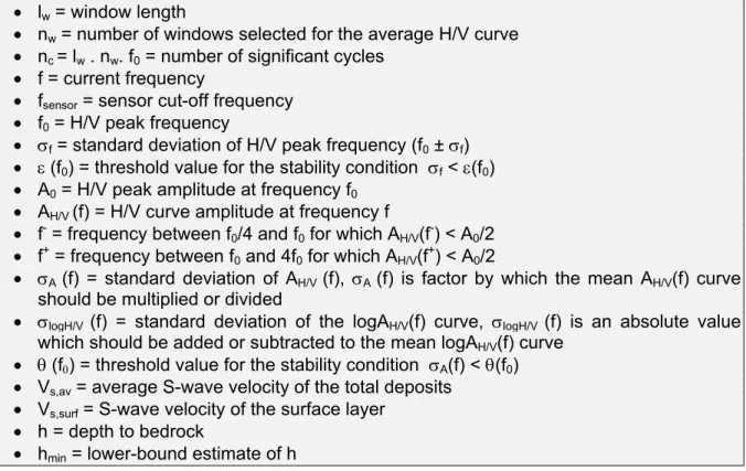
This section presents diagrams with criteria and recommendations to help in the result interpretation for different cases. For detailed explanations of each case, see section 3 in Part II of the guidelines. See Appendix A for illustrations. The definitions given in the table below are valid for all section 2.

2.1 Criteria for reliability of results

Criteria for a clear H/V peak

(at least 5 out of 6 criteria fulfilled)

i)

∃ f^-

∈ [f

0

/4, f

0

] | A

H/V

(f

^-

) < A

0

/2 ii)

∃ f⁺

∈ [f

0

, 4f

0

] | A

H/V

(f

⁺

) < A

0

/2 iii) A

0

> 2

iv) f

peak

[A

H/V

(f) ± σ

A

(f)] = f

0

±5%

v)

σf

< ε(f

0)

vi)

σA

(f

0

) < θ (f

0

)

• l_w = window length

• n_w = number of windows selected for the average H/V curve

• nc = lw . nw. f0 = number of significant cycles

• f = current frequency

• f_sensor = sensor cut-off frequency

• f₀ = H/V peak frequency

• σf = standard deviation of H/V peak frequency (f0 ± σf)

• ε (f₀) = threshold value for the stability condition σ_f < ε(f₀)

• A₀ = H/V peak amplitude at frequency f0

• AH/V (f) = H/V curve amplitude at frequency f

• f^- = frequency between f0/4 and f0 for which AH/V(f^-) < A0/2

• f⁺ = frequency between f0 and 4f0 for which AH/V(f⁺) < A0/2

• σA (f) = "standard deviation" of AH/V (f), σA (f) is the factor by which the mean AH/V(f) curve should be multiplied or divided

• σ_logH/V(f) = standard deviation of the logAH/V(f) curve, σ_logH/V(f) is an absolute value which should be added to or subtracted from the mean logAH/V(f) curve

• θ (f₀) = threshold value for the stability condition σ_A(f) < θ(f₀)

• V_s,av = average S-wave velocity of the total deposits

• Vs,surf = S-wave velocity of the surface layer

• h = depth to bedrock

• h_min = lower-bound estimate of h

Threshold Values for σf

and σ

A

(f

0

)

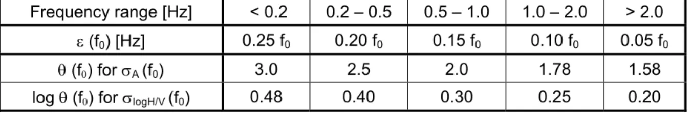
Frequency range [Hz] < 0.2 0.2 – 0.5 0.5 – 1.0 1.0 – 2.0 > 2.0 ε (f0) [Hz] 0.25 f₀ 0.20 f₀ 0.15 f₀ 0.10 f₀ 0.05 f₀

θ (f0) for σA (f₀) 3.0 2.5 2.0 1.78 1.58

log θ (f₀) for σ_logH/V(f₀) 0.48 0.40 0.30 0.25 0.20

Criteria for a reliable H/V curve i) f

0

> 10 / l

w

and

ii) n

c

(f

0

) > 200

and

iii)

σA

(f)<2

for 0.5f0<f<2f0 if f0>0.5Hz

or

σA

(f)<3

for 0.5f0<f<2f0 if f0<0.5Hz

2.2 Main peak types

This section is not an exhaustive list of the different types of H/V curves that might be obtained, but it gives suggestions for the processing and interpretation of the most common situations.

(11)

Sharp peaks and industrial origin

see $3.3.2.d and appendix A

If industrial origin is proved, i.e., if

♦ raw spectra exhibit sharp peaks on all omponents

c

♦ random decrement technique indicates very low damping (< 5%)

♦ peaks get sharper with decreasing smoothing

no reliable f

0

♦ Perform continuous recordings during day and night

♦ Check the existence of 24 h / 7 day plant within the area

If industrial origin is not obvious

Clear peak

see $3.3.1 and appendix A

If industrial origin ( $3.3.2.d ) , i.e.

♦ the raw spectra exhibit sharp peaks on all three components

♦ the random decrement technique indicates very low damping (< 5%)

♦ peaks get sharper with decreasing smoothing

f0 reliable

♦ Likely sharp contrast at depth (A0 > 4-5)

♦ f0 = fundamental frequency

♦ If h is known then VS,av ~ 4h.f0

♦ If V_S,surf is known then h_min~ V_S,surf/4f₀

If f

0

> f

sensor

and no industrial origin

no reliable f

0

(12)

Unclear low frequency peak

see $3.3.2.b and appendix A

If rock site

If steady increase of H/V ratio with decreasing frequency

♦ Check H/V curves from individual windows and eliminate windows giving spurious H/V curves

♦ Use longer time windows and/or more stringent window selection criteria

♦ Use proportional bandwidth and less smoothing

no reliable f

0

If reprocessed H/V curve does not fulfil the clarity criteria

f

0

reliable

Perform additional measurements over a longer time and/or during night and/or quiet weather conditions and/or use earthquake recordings using also a nearby rock site If reprocessed H/V curve fulfils the clarity criteria

Broad peak

see $3.3.2.c and appendix A

Decrease the smoothing bandwidth If bump peak is not stable and/or AH/V(f) is very large

♦ If clearer peaks are observed in the vicinity and

- if their related frequencies lie within the frequency range of the broad peak

- if their related frequencies exhibit significant variation from site to site

Then, examine the possibility of underground lateral variation, especially slopes.

♦ Otherwise not recommended to extract any information

no reliable f

0

If bump peak is stable and AH/V(f) is rather low

(13)

Multiple peaks (multiplicity of maxima) see $3.3.2.c and Appendix A

Check no industrial origin of one of the peaks Increase the smoothing bandwidth

If reprocessed H/V curve does not fulfil the clarity criteria

f

0

reliable

Redo measurements over a longer time and/or during night

If reprocessed H/V curve fulfils the clarity criteria

2 peaks cases (f

1

> f

0

)

see $3.3.2.d and appendix A

If the geology of the site shows possibility of having two large velocity contrasts at two different scales

AND

The clarity criteria are fulfilled for both f0 and f1

f0 and f1 reliable

♦ Likely two large contrasts at shallow and large depth at two different scales

♦ f1 = other natural frequency

♦ If VS,surf is known then h1,min ~ Vs,surf/4f1

If industrial origin of f₀ AND

No industrial origin for f₁

f0 not reliable and f1 reliable

♦ Likely sharp contrast at shallow depth

♦ If h is known then VS,av ~ 4h.f1

♦ If VS,surf is known then hmin ~ VS,surf/4f1

f0 reliable and f1 not reliable

♦ Likely sharp contrast at rather large depth

♦ If h is known then VS,av ~ 4h.fo

♦ If VS,surf is known then hmin ~ VS,surf/4fo

If industrial origin of f1

AND

No industrial origin for f0

(14)

Flat H/V curve (meeting the reliability conditions)

see $3.4 and appendix A

♦ Likely absence of any sharp contrast at depth

♦ Does not necessarily mean no amplification

♦ Perform earthquake recordings on site and nearby rock site

♦ Use of other geophysical techniques

if soil deposits

♦ likely unweathered or only lightly weathered rock

♦ may be considered as a good reference site

if rock

(15)

PART II: DETAILED TECHNICAL GUIDELINES

(16)

1. TECHNICAL REQUIREMENTS

It is important to understand which recording parameters influence data quality and reliability as this can help speed up the recording process. H/V measurements in cities are conducted within the following context:

– Anthropic noise is very high.

– It is quite rare to be able to get data on the soil per se. Most data will be obtained on streets and sidewalks (i.e. asphalt, pavement, cement or concrete), and to a lesser extent in parks (i.e. on grass or soil).

– Measurements are performed in an environment dominated by buildings of various dimensions.

– Recordings are not always performed at the same time and under the same weather conditions.

– The presence of underground structures (i.e. pipes,...) is often unknown.

The influence of various types of experimental parameter had to be tested on the results of H/V curves both in frequency and amplitude. For each tested parameter, H/V data were compared with a "reference situation". This comparison had to be made in an objective way, i.e. with the use of a statistical method. The Student-t test was chosen as it is one of the most commonly used techniques for testing an hypothesis on the basis of a difference between sample means. It determines a probability that two populations are the same with respect to the variable tested. The t-test can be performed knowing only the means, standard deviation, and number of data points. For further details, or for users who would like to perform some comparison on their own, please refer to the SESAME WP02 Controlled instrumentation specification, Final report. Further investigations would be welcome in some cases using a common software process and processing parameters to compare records and quantify their similarity.

This chapter is based on the following SESAME internal reports:

– WP02 Controlled instrumentation specification, Final report, Deliverable D01.02, – WP02 H/V technique : experimental conditions, Final report, Deliverable D08.02.

1.1 Instrumentation

An instrument workshop was held during the SESAME project to investigate the influence of different instruments in using the H/V technique with ambient vibration data. There were four major tasks performed, which consisted of testing the digitisers and sensors, and of making simultaneous recordings both outside in the free field and at the lab for comparisons.

Influence of the digitiser

In order to investigate the possible influence of the digitisers, several tests were performed to quantify the experimental sensitivity, internal noise, stability with time and channel consistency. The influence of various parameters was checked (warm up time, electronic noise, synchronism between channels, difference of gain between channels, etc.):

Æ Most of the tested digitisers finally gave correct results.

Æ In general it was found that all digitisers need some warm up time. From 2 to 10 minutes is usually sufficient for most instruments to assure that the baseline is more or less stable. Users are encouraged to test instrument stability before use.

Æ For an optimal analysis of the H/V curve, it appears to be necessary to check the energy density along the studied frequency band, to ensure that the energy is sufficient to allow the extraction of the signal from the instrumental noise. Furthermore, deviations must be the same on all components.

Æ Users should check synchronisation between channels: From numerical simulation, it was demonstrated that no H/V modification occurs below 15 Hz. Over 15 Hz modifications in the H/V results depend on the percentage of sample desynchronisation, the minimum being obtained for a round number of desynchronised samples and the maximum (up to 80% of H/V amplitude change) for 0.5 sample.

Æ Users should choose the same gain for all three channels. Small gain differences might cause slight changes to the results.

(17)

Influence of the sensor

The influence of the type of sensor was tested by recording simultaneously with two sensors coupled to the same digitiser. In total 17 sensors were tested. In general, signals are similar, as expected.

However,

Æ The accelerometers were not sensitive enough for frequencies lower than 1 Hz and give very unstable H/V results. It is not recommended that H/V measurements be performed using seismology accelerometers, as they are not sensitive enough for ambient vibration levels.

Æ Stability is important. It is not recommended that H/V measurements be performed using broadband seismometers (with natural period higher than 20 s), as they require a long stabilisation time, without providing any further advantage. Users are encouraged to test sensor stability before use.

Æ It is not recommended that sensors that have their natural frequency above the lowest frequency of interest be used. If f₀is lower than1 Hz, while the sensor used is a high frequency velocimeter, double check the results with the procedure indicated in 3.3.2.b.

1.2 Experimental conditions

As a general recommendation, it is suggested that before doing H/V measurements on the field, the team should have a look at the available geological information about the study area. In particular, the types of geological formations, the possible depth to the bedrock, and possible 2D or 3D structures should be looked at.

An evaluation of the influence of experimental conditions on the stability and reproducibility of H/V estimations from ambient vibrations was carried out during the SESAME project [2]. The results obtained are based on 593 recordings used to test 60 experimental conditions that can be divided into categories, as following:

– recording parameters, – recording duration, – measurement spacing, – in-situ soil-sensor coupling, – artificial soil-sensor coupling, – sensor setting,

– nearby structures, – weather conditions, – disturbances.

Recording parameters

Æ As long as there is no signal saturation, results are equivalent irrespective of the gain used. However, we suggest fixing the gain level at the maximum possible without signal saturation. The only noticeable effect is a compression of the H/V curve when too high a gain value is used implying too much saturation of the signal.

Æ A sampling rate of 50 Hz is sufficient, as the maximum frequency of engineering interest is not higher than 25 Hz, although higher sampling rates do not influence H/V results.

Æ Length of cable to connect the sensor to the station does not influence H/V results at least up to a length of 100 meters.

Recording duration

Æ In order for a measurement to be reliable, we recommend the following condition to be fulfilled : f0 > 10 / lw. This condition is proposed so that, at the frequency of interest, there be at least 10 significant cycles in each window (see Table 1).

Æ A large number of windows and of cycles is needed: we recommend that the total number of significant cycles : n_c= l_w . n_w .f₀ be larger than 200 (which means, for

(18)

instance, that for a peak at 1 Hz, there be at least 20 windows of 10 s each; or, for a peak at 0.5 Hz, 10 windows of 40 s each, or 20 windows of 20 s, but not 40 windows of 10 s). See Table 1 for other frequencies of interest.

As there might be some transients during the recording, these should be removed from the signal for processing, and the total recording duration should be increased, in order to have the above mentioned conditions fulfilled for "good quality" signal windows.

Table 1. Recommended recording duration.

f0 [Hz] Minimum value for lw [s]

Minimum number of significant

cycles (nc)

Minimum number of

windows

Minimum useful signal duration [s]

Recommended minimum record

duration [min]

0.2 50 200 10 1000 30'

0.5 20 200 10 400 20'

1 10 200 10 200 10'

2 5 200 10 100 5'

5 5 200 10 40 3'

10 5 200 10 20 2'

Measurement spacing

Æ For a microzonation, it is recommended that a large spacing be initially adopted (for example a 500 m grid) and, in case of lateral variation of the results, to densify the grid point spacing, down to 250 m, for example.

Æ For a single site response study, one should never use a single measurement point to derive an f₀ value. It is recommended that at least three measurement points be used.

In situ soil-sensor coupling

In situ soil / sensor coupling should be handled with care. Concrete and asphalt provide good results, whereas measuring on soft / irregular soils such as mud, grass, ploughed soil, ice, gravel, uncompacted snow, etc., should be looked at with more attention.

Æ To guarantee a good soil / sensor coupling the sensor should be directly set up on the ground, except in very special situations (steep slope, for example) for which an interface might be necessary (see next section).

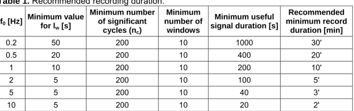
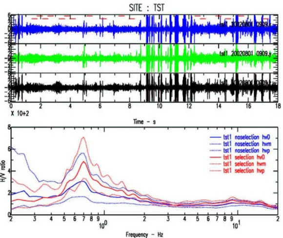
Æ Topping of asphalt or concrete does not affect H/V results in the main frequency band of interest, although slight perturbations can be observed in the 7-8 Hz range, which do not change the shape of the H/V curves. In the 0.2 – 20 Hz range, no artificial peaks are observed. Tests should be performed on higher frequency sites in order to check the influence of the asphalt thickness. See Figure 1 for a comparison with and without asphalt, at the same site.

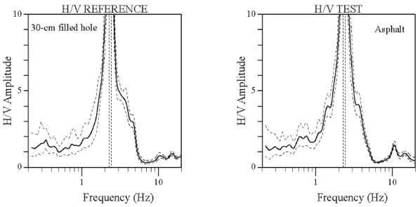
Æ Grass by itself does not affect H/V results, provided that the sensor is in good contact with the ground and not, for example, placed unstably on the grass as can be the case for tall grass folded under the sensor. In such cases, it is better to remove the high grass before installing the sensor, or to dig a hole in order to install the sensor directly on soil. Recording on grass when the wind is blowing can lead to completely perturbed results below 1 Hz, as shown on Figure 2.

Æ Avoid setting the sensor on superficial layers of "soft" soils, such as mud, ploughed soil, or artificial covers such as synthetic sport covering.

Æ Avoid recording on water saturated soils, for example after heavy rain.

(19)

Æ Avoid recording on superficial cohesionless gravel, as the sensor will not be correctly coupled to the ground and strongly perturbed curves will be obtained. Try to find another type of soil a few meters away, or remove the superficial gravel to find the firm ground below, if possible.

Æ Recording on snow or ice can affect the results. In such cases, it is recommended that the snow be compacted and the sensor installed on a metal or wood plate in order to avoid sensor tilting due to local melting under the sensor legs. When recording in such conditions, make sure that the temperature is within the equipment specifications given by the manufacturer.

Figure 1. Comparison of the H/V curves obtained with and without asphalt, at the same site, showing no significant effect of the asphalt layer.

Artificial soil-sensor coupling

When an artificial interface is needed between the ground and the sensor, it is highly recommended that some tests be performed before doing the recordings in order to examine a possible influence of the chosen interface.

Æ The use of a metal plate in-between the sensor and the ground does not modify the results.

Æ In case of a steep slope that does not allow correct sensor levelling, the best solution is to install the sensor on a pile of sand or in a plastic container filled with sand.

Æ In general, avoid "soft / non-cohesive" materials such as foam-rubber, cardboard, gravel (whether in a container or not), etc., to help setting up the sensor. See Figure 3 for a comparison with the sensor directly on the natural soil, or on a Styrofoam plate.

Sensor setting

Æ The sensor should be installed horizontally as recommended by the manufacturer.

Æ There is no need to bury the sensor, but it does not hurt if this is the case. It can be useful however, to set-up the sensor in a hole (no need to fill it) about its own size in order to get rid, for example, of the effect of a weak wind on grass. This would be effective only if there are no structures nearby, such as buildings or trees that might also induce some strong low frequency perturbations in the ground, due to the wind (see below).

(20)

Æ Do not put any load on the sensor.

Figure 2. Comparison of the H/V curves obtained at the same site on grass with and without wind (top), and in a hole, on asphalt (bottom) and again on grass with wind. This comparison shows the strong effect of the wind combined with grass, whereas on asphalt or in a hole, the wind has no significant effect (if far away from any structure).

(21)

Figure 3. Comparison of the H/V curves obtained with and without a Styrofoam plate under the sensor, at the same site, showing a strong effect of the Styrofoam.

Nearby structures

Æ Users are advised that recording near structures such as buildings, trees, etc., may influence the results: there is clear evidence that movements of the structures due to the wind may introduce strong low frequency perturbations in the ground. Unfortunately, it is not possible to quantify the minimum distance from the structure where the influence is negligible, as this distance depends on too many external factors (structure type, wind strength, soil type, etc.).

Æ Avoid measuring above underground structures such as car parks, pipes, sewer lids, etc., these structures may significantly alter the amplitude of the vertical motion.

Weather conditions

Æ Wind probably has the most frequent influence and we suggest avoiding measurements during windy days. Even a slight wind (approx. > 5 m/s) may strongly influence the H/V results by introducing large perturbations at low frequencies (below 1 Hz) that are not related to site effects. A consequence is that wind only perturbs low frequency sites.

Æ Measurements during heavy rain should be avoided, while slight rain has no noticeable influence on H/V results.

Æ Extreme temperatures should be treated with care, following the manufacturer's recommendations for the sensor and recorder; tests should be made by comparing night / day or sun / shadow measurements.

Æ Low pressure meteorological events generally raise the low frequency content and may alter the H/V curve. If the measurements cannot be delayed until quieter weather conditions, the occurrence of such events should be noted on the measurement field sheet.

Disturbances

Æ No influence from high voltage cables has been noted.

Æ All kinds of short-duration local sources (footsteps, car, train,...) can disturb the results.

The distance of influence depends on the energy of the source, on the soil conditions, etc., therefore it is not possible to give general minimum distance values. However, it has generally been observed, for example, that ambient vibration sources with short periods of high amplitude (e.g. fast highway traffic) influence H/V ratios if they are within 15-20 metres, but that more continuous sources (e.g. slow inner city traffic) only influence H/V ratios when they are much closer. Our experience is that it is the impulsiveness of the noise envelope that is crucial Therefore traffic is much less of a problem in a city than it is close to a highway, for example. Users are anyway encouraged to check recorded time series in the field when they perform measurements in a noisy environment.

Æ Short-duration disturbances of the signal can be avoided during the H/V analysis by using an anti-trigger window selection to remove the transients. A consequence is that the time duration of the recordings should be increased in order to gather enough duration of “quiet” signal (see sections 2 and 3), unless, for example, only one train has perturbed the recordings.

Æ Avoid measurements near monochromatic sources such as construction machines, industrial machines, pumps, etc.

Æ The recording team should not keep its car engine running during recordings.

(22)

2. DATA PROCESSING STANDARD: J-SESAME SOFTWARE

This chapter is based on the following SESAME internal reports:

– Multi-platform H/V processing software J-SESAME, Deliverable D09.03 [3], – J-SESAME User Manual, Version 1.07 [4],

J-SESAME is a JAVA application for providing a user-friendly graphical interface for the H/V spectral ratio technique, which is used in local site effect studies. The program uses the functions of automatic window selection and H/V spectral ratio by executing external commands. The automatic window selection and H/V process are standalone applications developed in Fortran. J-SESAME is mainly a tool for organising the input data, executing window selection and processing, and displaying the processing results. The software operates in Unix, Linux, Macintosh and Windows environments.

Details concerning system requirements and installation procedure are given in the J- SESAME user manual delivered with the software.

2.1 General design of the software

The general design of J-SESAME is based on a modular architecture. There are basically four main modules:

– browsing module,

– window selection module, – processing module, – display module.

The main functionalities are integrated through a graphical user interface, which is part of the browsing module. The display module is also tightly connected to the browsing module, as there is close interaction between the two modules due to the integrated code development in Java. Only two waveform data formats are accepted: GSE and SAF (SESAME ASCII Format), see J-SESAME user manual for more details.

2.2 Window Selection Module

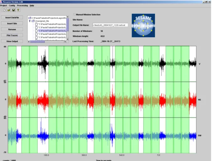
Windows can be selected automatically or manually. The manual window selection mode can be used if the check-box labelled as “Manual window selection” (Figure 4) is active.

Besides manual selection directly from the screen, which is often the most reliable, but also the most time consuming method, an automatic window selection module has been introduced to enable the processing of large amounts of data. The objective is to keep the most stationary parts of ambient vibrations, and to avoid the transients often associated with specific sources (footsteps, close traffic). This objective is exactly the opposite of the usual goal of seismologists who want to detect signals, and have developed specific "trigger"

algorithm to track the unusual transients. As a consequence, we have used here an

"antitrigger" algorithm, which is exactly the opposite: it detects transients but it tries to avoid them.

The procedure to detect transients is based on a classical comparison between the short term average "STA", i.e., the average level of signal amplitude over a short period of time, denoted "tsta" (typically around 0.5 to 2.0 s), and the long term average "LTA", i.e., the average level of signal amplitude over a much longer period of time, denoted "tlta" (typically several tens of seconds).

(23)

In the present case, we want to select windows without any energetic transients: this means that we want the ratio sta/lta to remain below a small threshold value smax (typically around 1.5 – 2) over a long enough duration. Simultaneously, we also want to avoid ambient vibration windows with abnormally low amplitudes: we therefore also introduce a minimum threshold smin, below which the signal should not fall during the selected ambient vibration window.

There are also two other criteria that may be optionally used for the window selection:

♦ one may wish to avoid signal saturation – as saturation does affect the Fourier spectrum.

As gain and maximum signal amplitudes are not mandatory in the header of SAF and GSE formats, the program looks for the maximum amplitude over the whole ambient vibration recording, and automatically excludes windows during which the peak amplitude exceeds 99.5 % of this maximum amplitude. By default, this option is turned on.

♦ in some cases, there might exist long transients (for instance related to heavy traffic, trains, machines, …) during which the sta/lta will actually remain within the set limits, but during which the ground motion may not be representative of real seismic ambient vibrations. Another option was therefore introduced to avoid "noisy windows", during which the lta value exceeds 80% of the peak lta value over the whole recording. By default, this option is turned off.

Figure 4. This figure shows the graphical user interface of J-SESAME. Selected windows are shown in green.

(24)

The program automatically looks for time windows satisfying the above criteria; when one window is selected, the program looks for the next window, and allows two subsequent windows to overlap by a specified amount "roverlap" (default value is 20%).

The window selection module has been written as an independent Fortran subroutine, for which:

♦ The input parameters are the selection parameters (tsta = STA window length; tlta = LTA window length; [smin, smax] = lower and upper allowed bounds for the sta/lta ratio; tlong

= ambient vibration window length over which the sta/lta should remain within the bounds; yes/no (1/0) parameters for turning on or off the saturation and "noisy window"

options; overlapping percentage allowed for two subsequent windows)

♦ The output parameters are the name of the ambient vibration file, the start and end times of each selected window, the recording status of each component : the main processing module then reads the ambient vibration file, and performs the H/V computation over each selected window.

Figure 5 shows an example where the same signal has been processed with and without the automatic window selection (that is the transient removal). This example shows that the peak on the H/V curve is much clearer when the transient removal is applied, and also that standard deviation is lower, especially at low frequencies.

Figure 5. Signal (top) processed with (red curves bottom) or without (blue curves bottom) the automatic window selection (selected windows are indicated by the red segments on the top of the signal). The peak on the H/V curve is much clearer when the transient removal is applied, and also the standard deviation is lower, especially at low frequencies.

(25)

The choice of the window selection parameters should be carefully optimised before any automatic processing.

2.3 Computing H/V spectral ratio

The main processing module is developed in FORTRAN90. It performs H/V spectral ratio computations and the other associated processing such as DC-offset removal, filtering, smoothing, merging of horizontal components, etc., on the selected windows for individual files or alternatively on several files as a batch process. The instrument response is assumed to be removed by the user (in the case of identical components H/V ratios should not be affected by the instrument response). Main functionalities of the processing module are described below:

♦ FFT (including tapering)

♦ Smoothing with several options. The Konno & Ohmachi smoothing is recommended as it accounts for the different number of points at low frequencies. Be careful with the use of constant bandwidth smoothing, which is not suitable for low frequencies.

♦ Merging two horizontal components with several options. Geometric mean is recommended.

♦ H/V Spectral ratio for each individual window

♦ Average of H/V ratios

♦ Standard deviation estimates of spectral ratios

Details of the different options are to be found in the Appendix of the J-SESAME User Manual. The parameter settings for the above options are controlled through an input file.

The processing module is applied according to the selected nodes in the tree. If the selected node is a site, then all the selected windows of the data-files collected for this site will be used for computing the average H/V spectral ratio. Output for each window can be also obtained by setting up the configuration parameters of the processing module. Batch processing will be performed when several sites or data-files are selected.

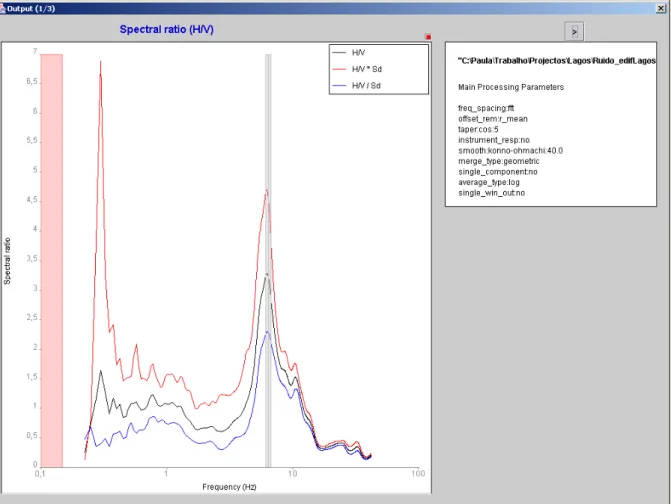
2.4 Showing output results

By pressing the <View Output> button (Figure 4) the user can navigate through three dialogue boxes. The first dialogue box (Figure 6) shows the H/V spectral ratio of the merged horizontal components, as well as the plus and minus one standard deviation curves. The second dialogue box shows the H/V spectral ratio for each one of the NS and EW components. The third one (Figure 7) shows the spectral ratio of the merged (H), NS and EW horizontal components and the spectra of V, NS and EW for each individual window, only if

“output single window information” is selected in the configuration parameter of the processing module.

(26)

Figure 6. H/V ratio for the merged horizontal components (mean in black, mean multiplied and divided by 10^σ^(logH/V), in red and blue). The pink strip shows the frequency range where the data has no significance, due to the sampling rate and the window length. The grey strip represents the mean f0, plus and minus the standard deviation. It is calculated from the f0 of each individual window.

2.5 Setting graph properties and creating images of the output results

For each graph shown (for example as in Figure 6 and 7) there is a small red box in the upper right corner without any label. By clicking there the properties and scale of the graph can be modified and images of the graph can be created. The button <Properties and series> pops up a dialogue box where line type, width and colour can be changed for each spectral curve. The button <Scales> pops up a dialogue box where the minimum, maximum and scale type for each one of the vertical and horizontal axes can be modified. The button

<Save> allows an image of the graph to be created.

(27)

Figure 7. Result for individual windows: H/V ratios and spectra shown are derived from the signal displayed in the red window.

(28)

3. INTERPRETATION OF RESULTS

Table 2. Definitions of the parameters used in this section.

• lw = window length

• nw = number of windows selected for the average H/V curve

• n_c= l_w . n_w. f₀ = number of significant cycles

• f = current frequency

• f_sensor = sensor cut-off frequency

• f₀ = H/V peak frequency

• σf = standard deviation of H/V peak frequency (f₀ ± σf)

• ε (f0) = threshold value for the stability condition σf < ε(f0)

• A0 = H/V peak amplitude at frequency f0

• AH/V (f) = H/V curve amplitude at frequency f

• f^- = frequency between f0/4 and f0 for which AH/V(f^-) < A0/2

• f⁺ = frequency between f₀ and 4f₀ for which A_H/V(f⁺) < A₀/2

• σ_A(f) = standard deviation of A_H/V(f), σ_A(f) is factor by which the mean A_H/V(f) curve should be multiplied or divided

• σlogH/V (f) = standard deviation of the logA_H/V(f) curve, σlogH/V (f) is an absolute value which should be added or subtracted to the mean logA_H/V(f) curve

• θ (f0) = threshold value for the stability condition σA(f) < θ(f0)

• Vs,av = average S-wave velocity of the total deposits

• Vs,surf = S-wave velocity of the surface layer

• h = depth to bedrock

• h_min = lower-bound estimate of h

3.1 Underlying assumptions

As detailed in Appendix B, the main information looked for within the H/V ratio is the fundamental natural frequency of the deposits, corresponding to the peak of the H/V curve.

While the reliability of its value will increase with the sharpness of the H/V peak , no straightforward information can be directly linked to the H/V peak amplitude A₀. This latter value may however be considered as indicative of the impedance contrasts at the site under study: large H/V peak values are generally associated with sharp velocity contrasts.

Figure 8 shows a comparison between the H/V ratio of ambient vibrations and the standard spectral ratio of earthquakes using a reference site. The comparison is performed using all the sites investigated in the framework of the SESAME project. The top part of the figure compares the value of the fundamental natural frequency f0 derived using both methods. An overall good agreement can be observed for the frequency values. The bottom part of Figure 8 compares the value of the peak amplitude A0. This comparison shows that it is not scientifically justified to use A0 as the actual site amplification. However, there is a general trend for the H/V peak amplitude to underestimate the actual site amplification. In other words, the H/V peak amplitude could generally be considered as a lower bound of the actual site amplification.

(29)

f0-H/V Ambient vibrations vs f0-SPR earthquakes

0 1 10

0 1

f0-SPR-earthquakes (Hz)

f0-H/V Ambient vibrations (Hz)

10

ANNECY BENEVENTO CATANIA CITTACASTELLO

COLFIORITO CORINTH EBRON EUROSEISTEST

FABRIANO GRENOBLE GUADELOUPE LOURDES

NICE PREDAPPIO ROVETTA TEHRAN

VERCHIANO VOLVI94 VOLVI97

A0-H/V Ambient vibrations vs A0-SPR earthquakes

0 1 2 3 4 5 6 7 8

A0-SPR-earthquakes

A0-H/V ambient vibrations

ANNECY BENEVENTO CATANIA

CITTAdiCASTELLO COLFIORITO CORINTH

EBRON EUROSEISTEST FABRIANO

GRENOBLE GUADELOUPE LOURDES

NICE PREDAPPIO ROVETTA

TEHRAN VERCHIANO VOLVI94

VOLVI97

Figure 8. Comparison between H/V ratio of ambient vibrations and standard spectral ratio of earthquakes. Top: comparison of the frequencies f₀, bottom: comparison of the amplitudes A₀.

(30)

The following interpretation guidelines are mainly linked with the clarity and stability of the H/V peak frequency value. The "clarity" however is related at least partly to the H/V peak amplitude (see below). While there are very clear situations where the risk of mistake is close to zero, one may also face cases (more than 50% in total) where the interpretation is uneasy and must call to some extent on "expert judgement": the following guidelines propose a framework for such an expert judgement, trying to minimise the subjectivity – which, however, can never be completely avoided.

3.2 Conditions for reliability

The first requirement, before any extraction of information and any interpretation, concerns the reliability of the H/V curve. Reliability implies stability, i.e., the fact that actual H/V curve obtained with the selected recordings, be representative of H/V curves that could be obtained with other ambient vibration recordings and/or with other physically reasonable window selection.

Such a requirement has several consequences :

i) In order for a peak to be significant, we recommend checking that the following condition is fulfilled : f₀ > 10 / l_w. This condition is proposed so that, at the frequency of interest, there be at least 10 significant cycles in each window (see Table 1). If the data allow – but this is not mandatory –, it is always fruitful to check whether a more stringent condition [ f₀ > 20 / l_w], can be fulfilled, which allows at least ten significant cycles for frequencies half the peak frequency, and thus enhances the reliability of the whole peak.

ii) A large number of windows and of cycles is needed: we recommend that, when using the automatic window selection with default parameters, the total number of significant cycles : nc = lw . nw .f0 be larger than 200 (which means, for instance, for a peak at 1 Hz, that there be at least 20 windows of 10 s each; or, for a peak at 0.5 Hz, 10 windows of 40 s each), see Table 1 for other frequencies of interest. In case no window selection is considered (all transients are taken into account), we recommend, for safety, this minimum nc number of cycles be raised around 2 times at low frequencies (i.e., up to 400), and up to 4 to 5 times at high frequencies, where transients are much more frequent (i.e., up to 1000).

iii) An acceptably low level of scattering between all windows is needed. Large standard deviation values often mean that ambient vibrations are strongly non-stationary and undergo some kind of perturbations, which may significantly affect the physical meaning of the H/V peak frequency. Therefore it is recommended that σA(f) be lower than a factor of 2 (for f0 > 0.5 Hz), or a factor of 3 (for f0 < 0.5 Hz), over a frequency range at least equal to [0.5f0, 2f0].

Therefore, in case one particular set of processing parameters does not lead to satisfactory results in terms of stability, we recommend reprocessing the recordings with some other processing parameters. As conditions for fulfilling items i , ii and iii above often lead to opposite tuning for some parameters (see section 2.), it may be impossible in some cases:

the safest decision is then to go back to the site and perform new measurements of longer duration and/or with more strictly controlled experimental conditions.

In addition, one must be very cautious if the H/V curve exhibits amplitude values very different from 1 (i.e., larger than 10, or lower than 0.1) over a large frequency range (i.e., over two octaves): in such a case, it is very likely that the measurements are bad (malfunction in the sensor or the recording system, very strong and close artificial ambient vibration sources, for instance), and should be redone ! It is mandatory to check the original time domain recordings first.

(31)

In the following interpretation guidelines, we assume that these reliability conditions are met;

if not, some reprocessing with other computational parameters should be attempted to try to meet them, or some additional measurements made. If none of these two options leads to satisfactory results, then the results should be considered with caution, and some reliability warning should be issued in the final interpretation.

3.3 Identification of f

0

3.3.1 Clear peak

The clear peak case is met when the H/V curve exhibits a "clear, single" H/V peak.

• The "clarity" concept may be related to several characteristics: the amplitude of the H/V peak and its relative value with respect to the H/V value in other frequency bands, the relative value of the standard deviation σA (f), and the standard deviation σf of f0

estimates from individual windows.

• the property "single" is related to the fact that in no other frequency band, does the H/V amplitude exhibit another "clear" peak satisfying the same criteria.

We propose the following quantitative criteria for the "clarity"

Amplitude conditions:

i) there exists one frequency f^-, lying between f₀/4 and f₀, such that A₀ / A_H/V (f^-) > 2 ii) there exists another frequency f⁺, lying between f₀ and 4.f₀, such that A₀ / A_H/V (f⁺) > 2 iii) A₀ > 2

Stability conditions:

iv) the peak should appear at the same frequency (within a percentage ± 5%) on the H/V curves corresponding to mean + and – one standard deviation.

v) σf lower than a frequency dependent threshold ε(f), detailed in Table 3.

vi) σ_A(f₀) lower than a frequency dependent threshold θ(f), also detailed in Table 3.

Table 3 gives the frequency dependent threshold values for the above given stability conditions v) σ_f < ε(f), and vi) σ_A(f₀) < log θ(f), or σ_logH/V(f₀) < θ(f).

Table 3. Threshold values for stability conditions.

Frequency range [Hz] < 0.2 0.2 – 0.5 0.5 – 1.0 1.0 – 2.0 > 2.0 ε (f0) [Hz] 0.25 f₀ 0.20 f₀ 0.15 f₀ 0.10 f₀ 0.05 f₀

θ (f0) for σA (f₀) 3.0 2.5 2.0 1.78 1.58

log θ (f0) for σlogH/V (f₀) 0.48 0.40 0.30 0.25 0.20

For the property "single", we propose that none of the other local maxima of the H/V curve fulfil all the above quantitative criteria for the "clarity".

If the H/V curves for a given site fulfil at least 5 out of these 6 criteria, then the f₀ value can be considered as a very reliable estimate of the fundamental frequency. If, in addition, the peak amplitude A₀ is larger than 4 to 5, one may be almost sure that there exists a sharp discontinuity with a large velocity contrast at some depth.

However, one has, in any case, to perform the two following checks:

(32)

• the frequency f₀ is consistent with the sensor cut-off frequency f_sensor and sensitivity : if f₀ is lower than1 Hz, while the sensor used is a high frequency velocimeter, check the results with the procedure indicated in 3.3.2.b.

• this sharp peak does not have an industrial origin (cf. 3.3.2.a).

Frequency statistics from individual windows Window

length lw [s]

Number of windows nw

Number of significant cycles nc

f0 [Hz] σ_f [Hz] A0 σ_A(f0)

41 14 1561 2.72 0.11 4.4 1.2

Figure 9. Example of a clear H/V curve, that fulfils all the criteria for "reliability" and "clarity"

given in sections 3.2 and 3.3.1.

3.3.2 "Unclear" cases

3.3.2-a Sharp peaks and Industrial origin

It often occurs in urban environments that H/V curves exhibit local narrow peaks – or troughs. In most cases, such peaks or troughs have an anthropic (usually industrial) origin, related to some kind of machinery (turbine, generators, ...).

Such perturbations are recognised by two general characteristics

• They may exist over a significant area (in other terms, they can be seen up to distances of several kilometres from their source).

• As the source is more or less "permanent" (at least within working hours), the original (non smoothed) Fourier spectra should exhibit sharp peaks .

Several kinds of checks are therefore recommended :

• Have a look at the raw spectra from each individual window : if they all exhibit a sharp peak (often on the 3 components together), at this particular frequency, there is a 95 % chance that this is anthropic "forced" ambient vibration and it should not be considered in the interpretation.

(33)

• Another check consists of reprocessing with less and less smoothing: in the case of industrial origin, the H/V peak should become sharper and sharper (while this is not the case for a "site effect" peak linked with the soil characteristics). In particular, checks with

"linear", "box" smoothing with smaller and smaller bandwidth should result in "box-like"

peaks having exactly the same bandwidth as the smoothing.

• If other measurements have been performed in the same area, determine whether a peak exists at the same frequencies with comparable sharpness (the amplitude of the associated peak, even for a fixed smoothing parameter, may vary significantly from site to site, being transformed sometimes into a trough).

• Another very effective check is to apply the random decrement technique (Dunand et al., 2002) to the ambient vibration recordings in order to derive the "impulse response"

around the frequency of interest: if the corresponding damping is very low (say, below 5%), an anthropic origin may be assumed almost certainly, and the frequency should not be considered in the interpretation.

• Whenever it is hard to reach a conclusion from the previous tests and this information is important, it is often very instructive to perform continuous measurements (over 24 h : day + night, or over one week: working days + week-end) to check whether these peaks also exist during non-working hours. There are, however, many plants that work 24h a day, 7 days a week: the test will not be conclusive in such a case, but it should be possible to identify such a plant with a minimum knowledge of the local industrial activity.

If any of the proposed checks does suggest an industrial origin, then the identified frequency should be completely discarded: it has no link with the subsurface structure.

Note : It may happen that the spurious frequency of industrial origin coincides with, or is not far from, a real site frequency. The existence of such artefacts may then alter the estimation of the actual site frequency f0; as much as possible, it is then preferable to perform measurements outside working hours to avoid this spurious peak, or to apply severe band- reject filters to the microtremor recordings in order to totally eliminate the artefact and its effects.

3.3.2-b Unclear low frequency peaks [criterion i) and possibly ii) not fulfilled]

There exist a number of conditions where the H/V curve exhibits a fuzzy, unclear low frequency peak (i.e., at frequencies lower than 1 Hz), or a broad peak that does not satisfy all the criteria above, especially the amplitude criteria.

It may have several origins (nonexclusive of one another)

• a low frequency site with either moderate impedance contrast (lower than approx. 4) at depth, or a velocity gradient, or a low level of low frequency ambient vibrations (for instance in continental areas)

• wind blowing during recording time, especially in the case of non-optimal recording conditions (for instance proximity of trees or buildings)

• measurements performed during a meteorological perturbation that may significantly enhance the low frequency content and alter the H/V ratio.

• a bad soil-sensor coupling, for instance on very wet soils (after rain), or with grass, or with a non-satisfactory plate