2D (as well as 1D) capability can handle supercritical and subcritical flow, as well as subcritical to supercritical and supercritical to subcritical flow transitions (hydraulic jumps). The 2D flow routing capabilities in HEC-RAS have been developed to allow the user to perform 2D or combined 1D/2D modeling. Within HEC-RAS Mapper, draw a boundary polygon for each of the 2D flow regions you want to model.
Connect 2D flow areas to 1D hydraulic elements (river reaches, side structures, storage area/2D flow area hydraulic connections) as needed. Enter all necessary boundary and initial condition data for the 2D flow zones in the unsteady flow data editor. Below is a list of current limitations of HEC-RAS 2D flow modeling software.
3 DEVELOPING A TERRAIN MODEL AND GEOSPATIAL LAYERS
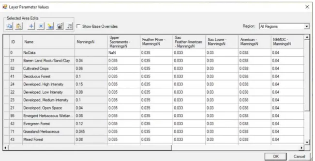
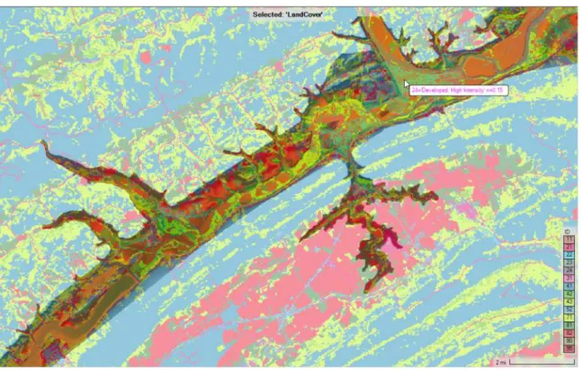
Once a land cover dataset is created, the user can specify Manning's n values to be used for each land cover type. RAS Mapper takes all input layers and creates a single output land cover layer in *.tif file format. You control the display of land use classification by right-clicking on the Land Cover layer and selecting Image Display Properties from the shortcut menu.
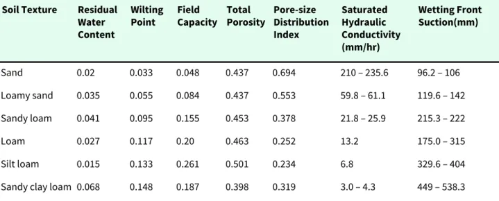
The user entered Manning's n values will be considered the base Manning's n values for this land cover layer. Once the user has created a land cover layer and added some of their own user defined ones. From the Infiltration Layer dialog (Figure 2-20), click the Create button to create a new raster layer that is the intersection of the ground cover and soil layers.
If no spacing is entered, it will automatically be set to the nominal cell size of the 2D flow area. To fix the mesh, simply delete the points that are outside the boundary of the 2D flow area. If the user chooses to associate the lateral structure with a 2D flow region, the lateral structure stationing is associated with the viewpoints of the 2D region.
The final step is to ensure that the face points of the 2D flow area are correctly connected to the stationing of the lateral structure. For this specific example, another additional lateral structure at the lower end of the 2D flow region will be added. The red line is what HEC-RAS uses to determine which part of the 1D cross section corresponds to the 2D Flow Area Faces.
Enter a time in hours for each of the 2D flow areas in the file labeled Initial Conditions Time (hours). The phase for the downstream 2D flow zone boundary is set to the computed phase of the 1D cross section each time step. The 2D flow field is being used to model the flow hydraulics downstream of the dam.
Draw the outer boundary of the 2D flow region all the way up to the other side of the hydraulic structure. Then select the editor Storage Area/ 2D flow area Hydraulic Connection (SA/2D Area Conn) in the left panel of the Geometric Data editor. Draw the upstream 2D flow area polygon right up to the edge of the hydraulic structure.
Draw the outer boundary of the 2D flow region downstream straight to the other side of the hydraulic structure. Next, select the Hydraulic Connection Storage Area/2D Flow Area (SA/2D Area Conn) editor in the left pane of the Geometric Data Editor. This cross section is automatically generated upstream of the bridge deck based on the user-entered Distance field (entered in the Deck/Bridge Path Data Editor).

5 BOUNDARY AND INITIAL CONDITIONS FOR 2D FLOW AREAS
In the example shown in Figure 4-1, two boundary lines of the flow region conditions have been entered on the right side of the 2D flow region. Once all 2D flow area boundary conditions (drawn with the SA/2D Area BC Lines tool) have been identified, the boundary condition type and boundary condition data (from the Unsteady Flow Data Editor) must be entered. As shown in Figure 4-2, the Select Location table below and then select Boundary Condition Type on the Boundary Conditions tab will contain all the boundary condition locations of the 2D flow region that have been entered in the Geometry Data Editor (Figure 4-1). .
Boundary condition lines can also be placed along other parts of the 2D flow area to allow flow to enter. When the elevation of the water surface of the step hydrograph is lower than the water surface in the 2D area of the flow, the flow will go out of the 2D area. The friction slope can be based on the slope of the land near the limit state line of the 2D flow region.
Next, the user must then select "Gridded" from the Mode Selection field in the Meteorological Variables section of the editor. The Ratio option allows the user to multiply all the precipitation by a user-specified ratio. Then, under the Meteorological Variables section of the editor, the user must select the point method from the Precipitation Mode drop-down menu.
For a Raster file data source, the user must specify the location and name of the file(s), as well as which group within the file contains the specific data (velocity or direction, X velocity, and Y velocity). The name of the 2D flow region will appear under the Initial Conditions tab of the Unsteady Flow Data Editor (see Figure 4-24). To use this option, enter the desired water surface height in the Initial Height column of the Unsteady Flow Data Editor, Initial Conditions tab, and in the 2D Flow Area row (see Figure 4-24).
For more information about the Restart File option, refer to the Unsteady Flow Data Editor section of the HEC-RAS Version 6.0 User Manual.
6 RUNNING A MODEL WITH 2D FLOW AREAS
Variable time step capabilities have been added to the unsteady flow engine for both a. The first option is a variable time step based on monitoring Courant numbers (or residence time inside a cell). These new variable Time Step options are accessed from the Unsteady Flow Analysis window (and also by going to the Calculation Options and Tolerances window).
The modified HEC-RAS Unsteady Computation Options and Tolerance window opens the new Advanced Time Step Control tab (Figure 5-3). The two new variable time step options (Courant number and Time Step Divisor) are discussed in the following sections. In the example shown in Figure 5-2 and Figure 5-3, the Courant number is used for the variable time step.
If the maximum number of Kurant is exceeded, then the time step is halved for the next time interval. For example, if the base calculation interval is 10 seconds and the user wants to allow it to go up to 40 seconds, then the value for this field would be 2 (ie, the time step can be doubled twice: 10 to 20 up to 40 seconds). The value displayed in the box to the right of the user-entered value is what will end up being the maximum time step entered.
If solving the equations gives a numerical answer that has less numerical error than the specified tolerance, then the solver moves to the next time step. This option allows the user to set a computational time step for a 2D flow region that is a part of the overall unsteady flow calculation interval. The Longitudinal Mixing Coefficient is used to calculate the contribution to the eddy viscosity from turbulence and dissipation in the longitudinal direction (ie, the flow direction).
If not, the calculated flow exchange will be reduced for the first guess of the flow rate for that time step.

7 VIEWING 2D OR 1D/2D OUTPUT USING HEC-RAS MAPPER
The user can create a terrain model from the cross-sections (channel only or entire sections), the river and bank lines and the cross-section interpolation surface. If the user is zoomed in, base (raw) data will be used to calculate the flood map layers; However, if the user zooms out, a re-sampled version of the terrain is used. Therefore, the displayed map layers may change slightly based on the scale at which the user is zoomed in.
The user has the option to create a "Stored" map layer (a grid stored on the hard drive) if desired. The Results Map Manager will then appear and the user can then select the Add New Map button from any of the plan names listed in this window to create a new Results Map layer. On the left is the map type where the user selects the parameter to be mapped (create a layer for).
For unsteady flow runs, the maximum value is the maximum depth times the velocity based on the user map interval, not the calculation interval. The maximum value is the maximum depth times velocity squared based on the user's map interval, not the calculation interval. The map output mode is where the user chooses whether the map will be a dynamic layer, created for the current view (in memory) or a saved map layer (saved to disk).
The Raster Gridded output is calculated based on user-specified Terrain and saved to disk. Once a map type, a transient profile, and a map output mode have been selected, the user then selects the Add Map button and the map will be added to the results layer under the selected plan. For dynamic depth results, the values reported to the user at a specific map location may vary depending on the zoom level.
This is because for dynamic mapping, the level of the terrain pyramid used to estimate the elevation of the land surface depends on how far the user has zoomed in or out on the map.