How rating agencies achieve rating stability

(1)

How rating agencies achieve rating stability

Edward I. Altman

^a,*

, Herbert A. Rijken

^b

aNYU Salomon Center, Leonard N. Stern School of Business, New York University, 44 West 4th Street, New York, NY 10012, USA

bVrije Universiteit Amsterdam, Faculty of Economics and Business Administration, De Boelelaan 1105, 1081 HV Amsterdam, The Netherlands

Available online 26 August 2004

Abstract

Surveys on the use of agency credit ratings reveal that some investors believe that rating agencies are relatively slow in adjusting their ratings. A well-accepted explanation for this perception on the timeliness of ratings is the through-the-cycle methodology that agencies use.

According to MoodyÕs, through-the-cycle ratings are stable because they are intended to measure default risk over long investment horizons, and because they are changed only when agencies are conﬁdent that observed changes in a companyÕs risk proﬁle are likely to be permanent.

To verify this explanation, we quantify the impact of the long-term default horizon and the prudent migration policy on rating stability from the perspective of an investor – with no desire for rating stability. This is done by benchmarking agency ratings with a ﬁnancial ratio-based (credit-scoring) agency-rating prediction model and (credit-scoring) default-prediction models of various time horizons. We also examine rating-migration practices. The ﬁnal result is a better quantitative understanding of the through-the-cycle methodology.

By varying the time horizon in the estimation of default-prediction models, we search for a best match with the agency-rating prediction model. Consistent with the agenciesÕstated objectives, we conclude that agency ratings are focused on the long term. In contrast to one-year default prediction models, agency ratings place less weight on short-term indicators of credit quality.

We also demonstrate that the focus of agencies on long investment horizons explains only part of the relative stability of agency ratings. The other aspect of through-the-cycle methodology – agency-rating migration policy – is an even more important factor underlying the

doi:10.1016/j.jbankﬁn.2004.06.006

* Corresponding author. Tel.: +1 212 998 0709; fax: +1 212 995 4220.

E-mail addresses:[email protected](E.I. Altman),[email protected](H.A. Rijken).

www.elsevier.com/locate/econbase

(2)

stability of agency ratings. We ﬁnd that rating migrations are triggered when the diﬀerence between the actual agency rating and the model predicted rating exceeds a certain threshold level. When rating migrations are triggered, agencies adjust their ratings only partially, consistent with the known serial dependency of agency-rating migrations.

JEL classiﬁcation:G20; G33

Keywords: Rating agencies; Through-the-cycle rating methodology; Migration policy; Credit-scoring models; Default prediction

1. Introduction

The credit ratings of MoodyÕs, Standard and PoorÕs, and Fitch play a key role in the pricing of credit risk and in the delineation of investment strategies. The future role of these agency ratings will be further expanded with the implementation of the Basle II accord, which establishes rating criteria for the capital allocations of banks.

Given the rather sudden meltdown in Asian countries and corporations in 1998 and the large increase in defaults in the 2001–2002 period, the timeliness of agency ratings has come under closer scrutiny and criticism.

A recent survey conducted by the Association for Financial Professionals (2002) reveals that most participants believe that agency ratings are slow in responding to changes in corporate credit quality.¹Surveys byEllis (1998)andBaker and Mansi (2002)report the same ﬁnding. The slowness in rating adjustments is well recognized by investors. Indeed, it seems that investors anticipate the well documented serial correlation in downgrades.²In a survey conducted byEllis (1998), 70% of investors believe that ratings should reﬂect recent changes in credit quality, even if they are likely to be reversed within a year. At the same time, investors want to keep their portfolio rebalancing as low as possible and desire some level of rating stability.

They do not want ratings to be changed to reflect small changes in financial condition. On the issue of two conflicting goals – rating timeliness and rating stability – investors appear to have ambiguous opinions. In their meetings with the institutional buyside in 2002, MoodyÕs repeatedly heard that investors value the current rating stability level and do not want ratings simply to follow market prices (see Fons et al., 2002).

The objective of agencies is to provide an accurate relative (i.e., ordinal) rank- ing of credit risk at each point in time, without reference to an explicit time horizon (see Cantor and Mann, 2003). In order to achieve rating stability, agencies take an undeﬁned long-term perspective, which lowers the sensitivity of

1 The critique of rating agencies focuses mainly on the timeliness of agency ratings, and not on the accuracy of agency ratings. The AFP survey reveals that 83% of the investors surveyed believe that, most of the time, agency ratings accurately reﬂect the issuersÕcreditworthiness.

2 This view has been echoed in a large number of conversations and interviews with market practitioners.

(3)

agency ratings to short-term fluctuations in credit quality. In their corporate ratings criteria document, Standard and PoorÕs (2003) takes the position that ‘‘the value of its products is greatest when its ratings focus on the long term and do not fluctuate with near term performance.’’³ Agencies aim to respond only to the perceived permanent (long-term) component of credit-quality changes. In addition, agencies follow a prudent migration policy. Only significant changes in credit quality result in rating migrations and, if triggered, ratings are partially adjusted.

The through-the-cycle rating methodology of agencies is designed to achieve an optimal balance between rating timeliness and rating stability.⁴The methodology has two key aspects: ﬁrst, a long-term default horizon and, second, a prudent migration policy. These two standpoints are aimed at avoiding excessive rating reversals, while holding the timeliness of agency ratings at an acceptable level.⁵It is unclear so far, which aspect of the through-the-cycle approach makes the primary contribution to rating stability.

So far details on how the through-the-cycle methodology is put into practice by agencies and quantitative details on its impact on rating stability are largely unknown to the outside world.⁶ The prime objective of this article is to shed some light in this black box. First we quantify the impact of the two aspects of the through-the-cycle methodology to rating stability from an investorÕs

3 In their disclosure on corporate ratings criteria, Standard and PoorÕs explains how to interpret their credit ratings (Standard and PoorÕs (2003), Corporate Ratings Criteria): ‘‘Standard and PoorÕs credit ratings are meant to be forward looking; that is, their time horizon extends as far as is analytically foreseeable. Accordingly, the anticipated ups and downs of business cycles – whether industry speciﬁc or related to the general economy – should be factored in the credit rating all along. This approach is in keeping with StandardÕs and PoorÕs belief that the value of its rating products is greatest when itÕs rating does not ﬂuctuate with near term performance. Ratings should never be a mere snapshot of the present situation. There are two models for how cyclicality is incorporated in credit ratings. Sometimes, ratings are held constant throughout the cycle. Alternatively, the rating does vary – but within a narrow band’’.

4 According to MoodyÕs, through-the-cycle methodology manages the tension between rating timeliness and rating stability: ‘‘If over time new information reveals a potential change in an issuerÕs relative creditworthiness, MoodyÕs considers whether or not to adjust the rating. It manages the tension between its dual objectives – accuracy and stability – by changing ratings only when it believes an issuer has experienced what is likely to be an enduring change in fundamental creditworthiness. For this reason, ratings are said toÔlook through the cycle.’’Õ(Cantor and Mann, 2003).

5 According to MoodyÕs, the optimal balance between rating stability and rating timeliness results from a close interaction between agencies and market participants: ‘‘In response to persistent market feedback, MoodyÕs manages its ratings with an eye towards minimizing abrupt changes in rating levels.’’ (Cantor, 2001).

6 There is no consensus on the details of the implementation of the through-the-cycle methodology.

Carey and Hrycay (2001)describe through-the-cycle methodology as a rating assignment based on a stress scenario. When firms are consequently rated in the bottom of the credit-quality cycle, agency ratings are insensitive to the credit-quality cycle and focus on the long term. An alternative interpretation of the through-the-cycle methodology is to extract the permanent component from changes in the observed credit quality, on the basis of a forecasting analysis: ‘‘Even though an issuer might experience a change in its financial performance as a result of an adjustment in the macroeconomic environment, its rating may nonetheless remain unchanged if it is likely that its previous financial condition will be restored during the next phase of the cycle.’’ (Cantor and Mann, 2003).

(4)

perspective – with no desire for rating stability, and second, we provide a further understanding of the through-the-cycle methodology by modeling the prudent migration policy. In order to measure rating stability we formulate credit-scoring models, reﬂecting the investorÕs perspective on credit quality. In a benchmark analysis, we compare the agency-rating dynamics with credit-model score dynamics. The conclusions of this study are useful to formulate policies to achieve an optimal balance between rating stability and rating timeliness, to provide guide- lines how to use agency ratings in the Basel II framework and to deﬁne conditions when it is acceptable to use agency-rating migration matrices as input to rating-based credit risk models.

Of crucial importance to this benchmark study is the formulation of a credible and accurate proxy for the investorÕs perspective on credit quality – with no desire for rating stability. For this purpose, credit-scoring default prediction models of various time horizons are estimated. We assume investors to have a point-in- time perspective on credit quality, comparable to the well documented perspective of banks. As opposed to through-the-cycle methodology, banks state that they base their internal ratings on the borrowerÕs current condition, i.e., current position in the credit quality cycle (see the Basel Committee on Banking Super- vision, 2000; Treacy and Carey, 1998). Their measures of the point-in-time credit quality reﬂect the current, possibly transient, market perception on credit quality.

As a consequence, banks examine both the permanent and transitory components of credit-quality changes. The extent to which point-in-time credit quality measures include temporary ﬂuctuations in credit quality depends on the default horizon. A large number of banks assess the credit quality with a one-year horizon, but nearly as many banks apply horizons of 3–7 years (see Basel Committee on Banking Supervision, 2000). In contrast to rating agencies, banks have no stated objective for rating stability or, more speciﬁcally, for avoiding rating reversals that could be caused by overreactions to temporary shocks. Agency ratings are aimed at ignoring temporary shocks and are therefore less likely to be reversed within a short period of time.

From the benchmark study we conﬁrm that agency ratings focus on predicting relative default risk over long horizons. We obtain this empirical ﬁnding by modeling the agency-rating scale with an ordered logit regression model and by modeling the default probability with a logit regression model for various time horizons. The agency-rating prediction model parameters closely match the parameters of a default-prediction model with a default horizon of 6 years.

A prudent migration policy is the second aspect of through-the-cycle methodology. The key issue of the migration policy is a reliable detection of the permanent (long-term) component in credit-quality changes and avoidance of rating reversals. Few details are known about the identiﬁcation of the permanent component by agencies. No straightforward method exists to forecast whether the nature of a credit-quality change is permanent or transitory. A combination of thorough analysis and expert judgment is needed to separate the permanent and transitory components. Because of the uncertainty inherent in forecasting

(5)

credit quality, agencies follow a prudent migration policy. We characterize the prudent migration policy by two parameters – a threshold parameter and an adjustment fraction parameter. First, a rating change is only considered by agencies if the actual rating differs significantly (by a specific threshold) from an estimated rating based on the most up-to-date credit quality information. Second, if triggered, the ratings are partially adjusted to the estimated rating. This partial adjustment is the source of serial correlation in agency-rating migrations, as reported by Altman and Kao (1991, 1992). Both the direction from which a rating class is reached and the time period of a stay in a particular class, are correlated with the following downgrade or upgrade intensity (see also Lando and Skøde- berg, 2002).

In a simulation experiment we quantify the two migration policy parameters. A rating migration is triggered when the rating predicted by a (credit-scoring) agency-rating prediction model diﬀers by at least a threshold level of 1.25 notch steps from the actual agency rating. If triggered, ratings are only partly adjusted, by about 75%. The rating adjustments are split and executed at diﬀerent times. Agencies appear to follow a moderate ‘‘wait-and-see’’ policy.

In the same spirit,Lo¨ffler (2002)examines a rating-migration policy model based on the idea that agencies try to avoid a rating bounce. In this model, agencies set different thresholds for each rating-migration step. The level of these thresholds is determined by a target rating bounce probability, which is set by the agencies and ideally kept as low as possible. Although the notions behind the modeling of agency-rating dynamics are similar to our model, the technical construction of our model differs. Instead of multiple thresholds, we include one threshold level at the upside and one at the downside. We further assume the ratings to be adjusted by a fraction to their predicted rating.⁷In addition, we apply a different simulation approach to test the validity of the rating-migration policy model. Instead of modeling credit-quality dynamics, we proxy the credit-quality dynamics by the dynamics of credit-model scores.

This paper proceeds as follows. In Section 2, the benchmark credit-scoring models are described. In this section the (credit-scoring) agency-rating prediction model is compared with (credit-scoring) default-prediction models for various time horizons.

Extensive attention is paid to the credibility of the estimated credit-scoring models to serve as a benchmark for agency ratings. Section 3 outlines the benchmark study.

Section 4 benchmarks agency rating dynamics and timeliness of agency-rating migrations. Section 5 describes the simulation experiment in which the migration policy parameters are quantiﬁed. Section 6 summarizes the consequences of the long-term default horizon and the prudent migration policy on agency-rating dynamics. Sec- tion 7 draws conclusions.

7 This adjustment fraction explains the serial correlation in agency-rating migration.Lo¨ﬄerÕs (2002) multiple threshold model explains rating drift as well. In a closely related paper,Lo¨ﬄer (2004)examines alternative explanations for rating drift. The partial rating adjustment hypothesis seems to be most convincing, however.

(6)

2. Benchmark credit-scoring models 2.1. Formulation of credit-scoring models

In our benchmark study, we examine the corporate-issuer credit ratings of Stand- ard and PoorÕs.⁸These ratings reﬂect ‘‘the obligorÕs ability and willingness to meet its ﬁnancial commitments on a timely basis’’ (see Standard and PoorÕs, 2003).

According to this deﬁnition, the corporate-issuer credit ratings of agencies are measures of default probability.

We formulate two benchmark credit-scoring models: a default-prediction model (DP model) and an agency-rating prediction model (AR model). Both the DP model and AR model employ the same model variables. This allows an unambiguous comparison of the dynamics of AR-scores and DP-scores. The estimation of these models diﬀers in the use of data (default events versus agency ratings) and statistical methodology.

At ﬁrst, the DP model is estimated for a short horizon of 1 year. The one-year default probability piis modeled as follows:

DP_i¼aþbXiþei; ð2:1Þ

log p_i 1p_i

¼DPi; ð2:2Þ

whereXiis the set of model variables for ﬁrm-year observationi. In a standard logit model setting, the error termseiare assumed to be identically distributed and inde- pendently distributed (Var(ei) =r², Cov(ei,ej) = 0 ifi5j). In reality, these error term conditions are violated. To obtain the correct statistics, Huber–White standard errors are used to relax the assumption of homoskedasticity. A generalization of these Huber–White standard errors (see Rogers, 1993) relaxes the assumption of independency among all observations as well. Instead, only independency among clusters of observations – a cluster includes all observations of the same ﬁrm – is assumed.

The parameters a, b are estimated by a maximum likelihood procedure. The DP- score is directly related to the one-year default probabilitypi.

The agency-rating prediction model (AR model) models the discrete agency-rating scale Nwith an ordered logit regression model. ⁹In this model, the AR-score (ARi) is an unobservable variable:

8 The empirical analysis is conducted using data on Standard and PoorÕs corporate-issuer credit ratings.

So, strictly speaking, the empirical results refer only to the ratings of Standard and PoorÕs. We are not aware, however, of a reason why the empirical results and the conclusions presented here for Standard and PoorÕs ratings should not apply for the ratings of MoodyÕs and Fitch. The discussions and conclusions in this article are therefore generalized to the agency ratings of Standard and PoorÕs and MoodyÕs and Fitch.

9 Bond ratings are modeled mainly for the purpose of forecasting agency-rating migrations (see for exampleEderington, 1985;Kaplan and Urwitz, 1979;Blume et al., 1998;Kamstra et al., 2001). Applied statistical methodologies are typically either ordinary least square analysis, ordered probit regression analysis, or discriminant analysis. In order to be consistent with the logit regression methodology of the default-prediction model, we model the agency ratings by an ordered logit model.

(7)

ARi¼aþbXiþei; ð2:3Þ whereXiis the set of model variables for ﬁrm-year observationi. The ARiscore is related to the agency rating kas follows:

y_i¼k if B_k1<AR_i6B_k; ð2:4Þ wherekis one of the agency-rating classes {CCC/CC, B, B,. . ., AA, AA+/AAA},¹⁰ yiis the actual agency rating,Bkis the upper boundary for the AR-score in rating class k, B0=1, and B16=1. In the ordered logit model, the probability thatyi

equalskis speciﬁed by:

Pðy_i¼kÞ ¼FðB_kARiÞ FðB_k1ARiÞ; ð2:5Þ where F is the cumulative logistic function. The parametersa, b, and Bk are estimated with a maximum likelihood procedure. As for the DP model, the generalized Huber–White standard errors are computed, thus relaxing the homoskedasticity assumption and the assumption of independency among observations of the same ﬁrm.

The AR-score is in fact a point-in-time measure of the long-term default risk view of agencies. It represents primarily one aspect of the through-the-cycle methodology, the long-term default horizon focus. The migration policy – the second aspect of the through-the-cycle methodology – has little impact on the estimation of the AR-model. The AR-scores might be slightly overstated but this does not eﬀect the benchmarking of ratingdynamics.

The slight overstatement of AR-scores is explained as follows. Due to a prudent migration policy, the agency ratings may be temporarily understated or overstated.

If the number of overstated ratings and the number of understated ratings – due to the prudent migration policy – are equal over the sample period, the migration policy will not aﬀect the AR-model estimate. In that case it will only widen the distribution of the error term e. However, the number of downgrades is 30% higher than the number of upgrades and the agency-rating migration shows a downward trend.

The number of overstated ratings is expected to be slightly higher and, as a consequence, the predicted ratings by the AR model are expected to be slightly higher than in absence of a prudent migration policy. This small shift in predicted rating level does not aﬀect the dynamic properties of these ratings.

2.2. Model variables in the credit-scoring models

The DP-score (Eq.(2.1)) and the AR-score (Eq.(2.3)) are calculated on the basis of the following set of six model variables:

10 In order to have a reasonable number of observations in each rating class, the agency-rating classes C, CC, CCC, CCC and CCC+ are combined to a single rating class CCC/CC, and the agency-rating classes AA+ and AAA are combined into a single rating class AA+/AAA.

(8)

DP-; AR-score¼aþb₁WK

TA þb₂RE

TAþb₃EBIT

TA þb₄ME

BLþb₅ Size

þb₆ Age; ð2:6Þ

where WK is net working capital, RE is retained earnings, TA is total assets, EBIT is earnings before interest and taxes, ME is the market value of equity, and BL is the book value of total liabilities. Size equals total liabilities normalized by the total value of the US equity market (Mkt) and log-transformed: ln(BL/Mkt). Age is the number of years since a firm was first rated by an agency.¹¹ In order to increase the effectiveness of the RE/TA, EBIT/TA and ME/BL variables in the logit model estimate, these variables are log-transformed as follows: RE/TA! ln(1RE/TA), EBIT/TA! ln(1EBIT/TA) and ME/BL!1 + ln(ME/BL). ¹²

The choice of the six model variables is inspired by the Z-score model (Altman, 1968).^13,14 The WK/TA variable is a proxy for the short-term liquidity of a ﬁrm.

The RE/TA, EBIT/TA, and ME/BL variables proxy for historic, current, and future profitability, respectively. The ME/BL variable also proxies for market leverage, which can be interpreted as the willingness of the stock market to invest in a particular firm. Multiple interpretations are possible for the ME/BL variable, as the market value of equity is a catchall variable of actual information regarding future earnings, confidence of investors et cetera. Empirical evidence of a ‘‘too-big-to-fail’’

11The Age variable is set to 10for observations with Age values above 10and for ﬁrms already rated at the start of the dataset in 1981.

12The distribution of the ME/BL variable is positively skewed. To a lesser extent, the distributions of the RE/TA variable and EBIT/TA variable are negatively skewed. The information content in the fat tails of the distributions is relatively low. For example, the difference between a ME/BL value of 50and 25 is far less informative than a difference between a ME/BL value of 1 and 0.5, which might distinguish a healthy firm from a firm approaching default. The effectiveness of the ME/BL variable in the logit regression model estimate can be improved by a log-transformation of the ME/BL variable:!1 + ln(ME/BL). This log-transformation stretches the informative part at the lower side of the ME/BL scale and compresses the non-informative part at the upper side of the ME/BL scale. For the same reason, the RE/TA and EBIT/TA variables are log-transformed:ln(1RE/TA) andln(1EBIT/TA). The log-transformation reduces the skewness in the distribution of these variables. The average value of these distributions is hardly affected, as the log-transformation centers around 1 for the ME/BL variable and around 0for the EBIT/TA and RE/TA variables.

13The sales-to-asset ratio is not included in the default-prediction model. This variable adds little additional value to a default-prediction model when estimated for a sample of ﬁrms covering a wide range of industries.

14In a report on their rating methodology,Standard and PoorÕs (2003)describes a set of 8 key ratios.

These ratios include two interest coverage ratios, two cash flow ratios, two earnings profitability ratios and two leverage ratios. In numerous empirical studies on credit-scoring models, different sets of variables are proposed to proxy for these four groups of credit-risk fundamentals. In general, interest coverage ratios and cash flow ratios appear to add surprisingly little to the explanation of default. The strong correlation of these variables with earnings profitability and leverage presumably prevents a significant marginal contribution. Moreover, interest coverage ratios often suffer from ambiguity problems, as both the denominator values (interest) and numerator values (EBIT) are centered close to 0. Only the profitability and leverage ratios, therefore, are included in the benchmark credit-scoring models.

(9)

default protection,¹⁵ and empirical evidence of a strong negative relationship between Age and the default rate (for Age values below 10)¹⁶motivate the inclusion of Size and Age variables in the credit-scoring models.

We do not try to find an optimal set of model variables in the logit model. First, it would be beyond the scope of this article to replicate the numerous studies on finding an optimal set of model variables.¹⁷Second, the Z-score variables have a good track record. Third, we believe that variation in proxies for profitability and leverage could improve the effectiveness of the credit-scoring models only marginally.

2.3. Parameter estimates of the credit-scoring models

Data on agency ratings is obtained from the Standard and PoorÕs CREDITPRO database, the July 2002 version, which includes all S&P corporate credit ratings in the period January 1981–July 2002. Less than half of the data in CREDITPRO can be linked with COMPUSTAT data.¹⁸The requirement of stock price data avail- ability restricts the sample to public firms. In addition, only non-financial US firms are selected.

The panel dataset covers the 1981–2001 period and includes the time series of 1772 obligors with period lengths between 1 and 21 years. It contains 11,890ﬁrm- year observations with known S&P ratings and 1828 ﬁrm-year observations with

15 Although the size of total market equity is often included in default-prediction models, this variable strongly correlates with the ME/BL variable. We include the size of total liabilities instead. Apart from this technical reason, the size of total liabilities is more directly related to the too-big-to-fail protection. One explanation for the too-big-to-fail protection is that credit holders might shy away from the large potential losses in case of a default or bankruptcy, hoping that the problems will be solved by time. The potential loss of large loans, potential damage to bank reputations, and the number of credit holders involved may all slow down the decision process, thereby allowing more time for companies with larger loans to restructure themselves.

16 A strong negative relationship exists between the Age variable and the default rate for Age values below 10. An exception forms the low default rate in the first year after being rated for the first time (Age = 1); that is, the so-called aging or mortality factor documented inAltman and Bana (2003). This suggests a need for a dummy variable. In a multivariate logit model estimate, however, the parameter of this dummy variable is not statistically significant. The lower default rate in the first year is probably captured by the healthier financial ratios. New ratings often coincide with bond issues, which enhance the financial condition of the issuing firms, at least temporarily.

17 Most of the literature on credit-scoring models was written in the seventies and the eighties. Research on credit-scoring models has recently gained renewed interest for two reasons. First, the record high default rates in the years 2001 and 2002 (e.g.,Altman and Bana, 2003) stimulated a further improvement and reﬁnement of these models. Second, the expected implementation of the Basle II accord has triggered eﬀorts to upgrade internal rating systems of banking institutions.

18 Apart from minor deviations, the distribution in S&P ratings is not aﬀected by this data reduction and selection of public ﬁrms. The percentage of defaulting observations at the beginning of the nineties shrinks, however, while the percentage of defaulting observations in the years 2000 and 2001 increases.

Presumably, the credit quality of public firms is less affected than that of private firms by the recession in the beginning of the nineties. In the years 2000 and 2001, the opposite occurred.

(10)

non-rated S&P status.¹⁹ Each ﬁrm-year observation consists of the S&P rating at the end of June and the values of the model-variables known to the public at that date. Market equity values are based on stock price and total shares outstanding at the end of June. To ensure that the accounting information is publicly available, all balance sheet data refer to the latest ﬁscal quarter in the previous calendar year.

The income statement data refer to the four fiscal quarters in the previous calendar year. ²⁰This six-month lagging condition for accounting information may be some- what conservative, as most accounting data become available in the first months after the end of a fiscal year/quarter. For troubled firms, however, financial information is, in general, slower in reaching the financial community.

The panel observations are split into surviving observations and defaulting observations. For the 13,447 surviving observations, stock price data are available both at the end of June in the current year and at the end of June in the subsequent year.²¹ For the 271 defaulting observations, the default event happens in the subsequent year. ²² The dependent binary variable pi in the logit-regression model estimation (see Eq. (2.2)) is equal to 1 for surviving observations and 0for defaulting observations.

Table 1provides mean and median values for the model variables, after truncation of their most extreme values.²³ The log-transformations of the ME/BL, RE/

TA and EBIT/TA variables reduce the skewness in their panel distributions considerably. The panel distribution of the log transformed ME/BL variable approaches a normal distribution.

19The reason to include panel observations of ﬁrms with a S&P non-rated status in the estimation of the DP model is to maximize the number of observations in the default-prediction model estimate. Firms with a non-rated status are monitored for default events as well. When defaulting, the rating status of ﬁrms with a non-rated status changes to D status.

20For companies whose fiscal years end in December, the accounting information refers to the previous fiscal year which equals the previous calendar year. For about 30% of the companies, the fiscal year does not end in December. For these companies the (approximately) six-month lagging accounting information at the end of June is derived as follows: the income statement data are averaged for the four fiscal quarters ending in the previous calendar year. In addition, the balance sheet data are taken from the latest-ending fiscal quarter in the previous calendar year.

21The surviving observations are observations of firms at the end of June in yearXthat also have stock exchange listings at the end of June in yearX+ 1. This imposes a survivorship bias. Robustness tests show that this bias does not significantly affect the parameter estimates of the benchmark models.

22The defaulting observations are observations of ﬁrms at the end of June in yearXthat default between the end of June in yearXand the end of June in yearX+ 1.

23The raw COMPUSTAT data produce some extreme values for the model variables that contain little relevant information. In order to reduce the impact of these observations the 0.5% highest values and the 0.5% lowest values are truncated for each model variable. These values are replaced by values ranked at 99.5% and 0.5%, respectively. Even though defaults are extreme events, a little amount of defaulting observations is aﬀected by this truncation procedure.

(11)

The DP model parameters are estimated for the period 1981–1999 (see the ﬁrst column of Table 2). The signs of all estimated parameters match expectations.

The ME/BL variable turns out to be the dominant variable in the DP model.²⁴This is consistent with the success of MoodyÕs KMV structural model, in which market equity and total liabilities play a key role. Although the ME/BL variable is the most important variable, accounting and ﬁrm-descriptive information – particularly the obligor characteristics of Size and Age – add substantially to the explanation of the incidence of default.

Table 1

Descriptive statistics for the model variables included in the credit-scoring models Agency rating N WK/TA

(4–5)/6

RE/TA ln(1–36/6)

EBIT/TA ln(1–178/6)

ME/BL 1 + ln(ME/181)

Size ln(181/Mkt)

Age

Mean statistic per rating class

AAA 317 0.15 0.64 0.17 1.98 6.53 9.14

AA 1198 0.12 0.52 0.14 1.67 7.51 9.07

A 2885 0.14 0.39 0.12 1.35 7.97 8.72

BBB 2603 0.14 0.27 0.10 1.05 8.48 7.77

BB 2396 0.18 0.11 0.09 0.82 9.37 6.01

B 2323 0.22 0.03 0.04 0.56 10.05 5.29

CCC/CC 168 0.08 0.21 0.05 0.66 10.08 5.45

NR 1828 0.26 0.21 0.08 1.28 10.55 9.06 Mean of observations 1 year preceding default (1 Y before D) and at default (D)

1 Y before D 271 0.11 0.17 0.02 0.83 10.02 5.33

D 167 0.13 0.45 0.07 2.44 9.86 5.88

Statistics for all 13,718 panel observations (excluding D ratings)

Mean 13,718 0.17 0.23 0.092 1.07 8.95 7.53

Median 13,718 0.15 0.20 0.092 1.08 9.05 10

Std. dev. 13,718 0.19 0.35 0.087 1.11 1.66 3.37

Min 13,718 0.51 1.22 0.33 3.78 15.04 1

Max 13,718 0.73 1.56 0.40 4.16 3.18 10

Kurtosis 13,718 3.36 5.68 7.13 3.83 2.89 2.04

Skewness 13,718 0.42 0.03 0.42 0.22 0.20 0.86

The table presents descriptive panel data statistics for the model variables in the credit-scoring models. The dataset consists of 13,718 observations from the period 1981–2001, including 271 observations of firms less than 1 year before default (1 Y before D). For the period after the default event, sufficient data on the model variables are available for 167 of the defaulted firms (D). WK is net working capital, RE is retained earnings, TA is total assets, EBIT is earnings before interest and taxes, ME is the market value of equity, and BL is the book value of total liabilities. Size equals total liabilities, normalized by the total value of the US equity market (Mkt). Age is the number of years since a firm was first rated by an agency. The numbers in the first row refer to COMPUSTAT data codes. The variables RE/TA, EBIT/TA, ME/BL, and Size are log transformed as indicated in the table.

24 A logit model that excludes the ME/BL variable is less eﬀective in explaining default rates than is a logit model that includes only the ME/BL variable. Including the ME/BL variable in the logit model reduces the weights of the EBIT/TA variable and the RE/TA variable considerably.

(12)

Because of the arbitrary nature of the DP model, the robustness of the estimated DP parameters is extensively tested.

Table 2

Parameter estimates for the DP and the AR model

Default-prediction model (logit model)

Agency-rating prediction model (ordered logit model) 1981–1999 2000–2001 1981–1999 2000–2001

Const 7.06 0.68 – –

(9.35) (0.76)

WK/TA 0.41 1.37 1.80 1.71

(0.75) (2.11) (6.27) (4.39)

RE/TA 0.20 0.89 3.33 2.84

(0.58) (1.94) (16.48) (10.59)

EBIT/TA 3.78 8.36 4.708.11

(3.79) (5.76) (8.70) (9.80)

ME/BL 1.28 1.01 0.85 0.52

(12.83) (9.73) (15.89) (11.15)

Size 0.47 0.24 0.95 0.93

(6.40) (2.84) (17.59) (14.78)

Age 0.20 0.14 0.082 0.082

(6.83) (3.63) (6.76) (4.02)

Boundaries Bk

AAA/AA+ – – 0.24 0.26

AA – – 1.61 0.69

AA – – 2.25 1.51

A+ – – 3.06 2.53

A – – 4.14 3.66

A – – 4.73 4.31

BBB+ – – 5.30 5.04

BBB – – 5.99 5.79

BBB – – 6.55 6.53

BB+ – – 7.01 7.00

BB – – 7.64 7.73

BB – – 8.56 8.78

B+ – – 10.31 10.15 B – – 11.65 11.52 B – – 13.05 12.93

CCC/CC – – 1 1

Pseudo-R² 0.355 0.374 0.214 0.231

Nobservations 119901728 10345 1545

Nobs. 1 year preceding default 150121 – –

The table presents the parameter estimates for the DP and the AR model. The dependent binary variable in the logit regression model estimation is 0for the defaulting observations (firms defaulting within 1 year) and 1 for all surviving observations (firms surviving in subsequent year). The dependent variable in the ordered logit regression model estimation is the agency-rating scale. The standard errors in the logit regression estimation are a generalized version of the Huber and White standard errors, which relaxes the assumptions concerning the distribution of error terms and independence among observations of the same firm. Thez-statistics are given in brackets. The pseudo-R²is a measure for the goodness of the fit.

(13)

• For two sub-periods, 1981–1990and 1991–1999, the DP parameters largely agree with each other, thus demonstrating the time stability of the DP model for the entire 1981–1999 period. Observations in the period 2000–2001 are excluded from the estimation of the DP model. In this period, the DP parameters differ significantly from the period 1981–1999 (see Table 2). The EBIT/TA variable has become more informative on credit quality. Furthermore, the too-big-to-fail default protection has disappeared. Instead, firms with large Size values experienced a higher default rate; 90firms with liabilities greater than $1 billion defaulted over the 30-month period between January 2001 and June 2003 (seeAlt- man and Bana, 2003). We must wait to determine whether these abrupt changes in DP parameters represent a regime change or should be ascribed to temporally exceptional circumstances. Notice that a large number of large liability failures have occurred in the telecommunications sector.

• When controlling for industry diﬀerences, the DP parameters change only slightly, 20% at most. By exception, the estimated parameter of the WK/TA variable increases to a signiﬁcant value of 0.94. When estimating the DP model separately by industry, the DP parameters are largely comparable.²⁵

• To ensure that the DP parameters are not related either to this particular S&P corporate bond dataset or the Standard and PoorÕs deﬁnition of default, the DP model is re-estimated for all bankruptcies, reported by COMPUSTAT.²⁶ The Age variable is omitted in this re-estimation. Due to space considerations, these results are not presented in this article.²⁷ The relative weights of the DP parameters appear to be robust to the choice of dataset and the deﬁnition of the default event. When using the bankruptcy dataset, the relative weight of the DP parameters is stable over time, varying at the most by 20% between the two sub-periods 1970–1980 and 1981–1998. This allows the DP model to be considered as an out-of-sample model for the entire period 1981–2001.

In summary, for the period 1981–1999, the DP model is stable over time and robust to the definition of default and to dataset choice. It is applicable for different industry sectors and obligors of different sizes. This emphasizes the universal charac- ter that makes the DP model a suitable benchmark for agency ratings (excluding the financial sector).

The AR parameters are estimated for the period 1981–1999 (see third column of Table 2). All parameter estimates have the expected sign. ²⁸ As are the DP parameters, the AR parameters are robust to a split in sample period: 1981–1990

25 The DP model is estimated separately for six industry sectors, defined by the first digit of the SIC code. The sign of the estimated parameters does not vary; the magnitude of the parameters varies within a factor two among these six industry sectors. The parameter for the WK/TA variable is an exception to this finding. It appears to be significantly positive for the infrastructure services sector.

26 The bankruptcy dataset covers the 1970–1998 period and contains 118,154 surviving observations and 755 bankruptcy observations. Only a small percentage of these bankruptcy observations overlap the defaulting observations in the Standard and PoorÕs corporate bond dataset.

27 Results are available on request.

28 The WK/TA variable is an exception.

(14)

and 1991–1999. Observations from 2000 and 2001 are excluded from this model estimation as well, as the AR parameters for this period diﬀer for the EBIT/TA and ME/

BL variables (seeTable 2). The AR parameters are robust to a split of observations into non-investment graded (BB+ and below) ﬁrms and investment graded (BBB and above) ﬁrms.²⁹This allows to model the entire agency-rating scale with one single parameter set.

2.4. Identifying the time horizon of the agency-rating prediction model

While the DP model has a known one-year horizon by construction, the AR model has no immediately identiﬁable time horizon. In order to measure the implicit time horizon of the AR model, we compare the AR parameters with those of the long-term default-prediction models (LDP models).

As for the DP model, the LDP models are estimated with a logit-regression model (see Eqs.(2.1) and (2.2)). The only difference between the DP model estimation and the LDP model estimation is the definition of surviving observations (pi= 1) and defaulting observations (pi= 0). For a given time horizon T, surviving observations are observations of firms surviving beyond T years, and defaulting observations are observations of firms defaulting within Tyears. The LDP score represents the probability of default in the comingTyears.

LDP models are estimated for a four-year and a six-year horizon. The parameters of these models are estimated for the period 1981–1995 (see Table 3).³⁰The generalized version of the Huber and White standard errors accounts for the overlapping periods in the estimation of the LDP model.³¹

The relative weights of the model variables in the AR, DP, and LDP models are compared using the following formula:

RWi¼ jb_ijri

P6 j¼1jb_jjrj

; ð2:7Þ

where RWiis the relative weight of model variablei,biis the parameter estimate for model variablei, andriis the standard deviation in the panel distribution of model variable iin the period 1981–1995.

29The only major difference is the absence of a significant parameter for the Age variable for non- investment grade firms.

30For comparability reasons, all models presented inTable 3are estimated for the sample period 1981–

1995. In this case, each ﬁrm-year observation can ‘‘look’’ 6 years ahead. Including observations in years after 1995 would lower the eﬀective time horizon.

31Unlike the DP model, the LDP model models multiyear cumulative default rates. Observations of the same firm are not only correlated because of the relative stable credit quality position over time, but also because of the overlapping multiyear periods in the definition of defaulting observations and surviving observations. Because of their time robustness, the estimated DP parameters and AR parameters hardly differ between an estimation period 1981–1999 (Table 2) and 1981–1995 (Table 3).

(15)

The ME/BL variable dominates in the DP model with a RW value of 41.7%. The Size and Age variables have substantial RW values in the DP model as well. These three variables account for most of the variation in the DP-score. The WK/TA, RE/

TA, and EBIT/TA variables play only a minor role. The AR model gives the most weight to the Size, RE/TA and ME/BL variables. The RW values of the AR model

Table 3

Comparison of the DP, LDP, and AR models

DP model LDP model AR model

Default-prediction time horizon: 1 year 4 years 6 years – Regression results

Constant 7.72 7.06 6.84 6.77^a

(8.36) (7.74) (8.06) (0.56)

WK/TA 0.00 0.56 0.82 1.85

(0.00) (1.01) (1.53) (5.36)

RE/TA 0.52 0.70 1.12 3.58

(1.04) (1.91) (3.21) (15.68)

EBIT/TA 3.61 3.31 1.57 4.49

(2.46) (2.83) (1.30) (7.48)

ME/BL 1.34 1.09 0.93 0.94

(8.71) (9.68) (8.54) (14.23)

Size 0.51 0.64 0.66 1.00

(5.44) (6.89) (7.44) (15.20)

Age 0.183 0.179 0.151 0.080

(4.89) (5.31) (4.82) (5.57)

Pseudo-R² 0.347 0.326 0.304 0.213

# surviving obs. 8639 7424 6782 7419

# default obs. 83 293 400 –

Relative weight model variables RW

WK/TA 0.0% 3.1% 4.8% 7.3%

RE/TA 5.2% 6.9% 11.8% 24.7%

EBIT/TA 8.9% 8.0% 4.0% 7.6%

ME/BL 41.7% 32.9% 29.8% 20.1%

Size 25.7% 31.5% 33.9% 34.7%

Age 18.5% 17.6% 15.7% 5.6%

The table presents the parameter estimatesaandb(see Eqs.(2.1) and (2.3)) and the relative weight RW of the model variables (see Eq.(2.7)) for the DP model, the LDP models, and the AR model. In case of the LDP models, the dependent binary variable in the logit regression model estimation is 0for the defaulting observations (firms defaulting within the default prediction time horizon) and 1 for all surviving observations (firms surviving within the default prediction time horizon). The parameters and RW values are estimated for the period 1981–1995. The standard errors in the logit regression estimation are a generalized version of the Huber and White standard errors, which relaxes the assumptions concerning the distribution of error terms and independence among observations of the same firm. Thez-statistics are given in brackets. The pseudo-R²is a measure for the goodness of the fit.

a Due to space considerations, only the estimated boundary between the rating category BB+ and BBB(B7, see Eq.(2.4)) is shown. In this particular case, the standard error of this boundary value is given in the brackets.

(16)

match most closely with the RW values of the six-year LDP model. This conﬁrms the long term perspective of agency ratings.

Especially for the RE/TA and ME/BL variables, a clear shift in relative weight is observed in the DP, LDP, and AR models, in that order (see Table 3). ³² Not surprisingly, the short-term oriented DP model depends heavily on variables which follow most closely the business cycle, like ME/BL. The AR model and LDP model place relatively more weight on variables which are less sensitive to business cycles, like historical earnings and Size. The traditional measures of ‘‘fundamental’’ risk dominate in long-term measures of credit risk. In the short term, however, if a ﬁrm is valued poorly in the marketplace and needs cash to avoid default, it will default.

In the remainder of this article the AR model will refer to the model estimate of the agency-rating scale in the period 1981–1999 (seeTable 2), the DP model will refer to the model estimate of the one-year default probability in period 1981–1999 (see Table 2), and the LDP model will refer to the model estimate of the six-year default probability in period 1981–1995 (see Table 3). CM-scores refer in general to AR- scores, LDP-scores and DP-scores. The benchmark analysis itself covers the period 1981–2001.

2.5. Matching CM-scores with agency ratings

In order to examine the credibility of AR-scores and DP-scores to serve as a benchmark for agency ratings, the CM-scores are matched with agency ratings.

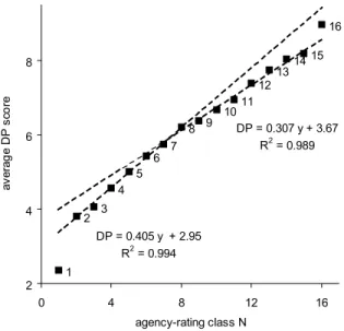
Average AR-scores and average DP-scores are computed for each agency-rating class. In Fig. 1, these average values are plotted against a numerical agency-rating scale N: CCC/CC/C = 1, B= 2, B = 3, B+ = 4,. . ., AA= 14, AA = 15, and AA+/

AAA = 16. This numerical rating scale is an arbitrary, but quite intuitive, choice that is commonly found in the mapping of bank internal-rating models to agency ratings.

The relationship between average DP-score and agency ratingNis close to linear.

Apparently, the DP-scores are suﬃciently and nearly equally dispersed over the entire agency-rating scale. On a more detailed level, two groups of rating classes with an almost perfect linear relationship can be distinguished (DP =a+cN+e). For non- investment rating classes 2–7, the slopecequals 0.405. For investment rating classes 8–15, the slopecequals 0.307 (seeFig. 1).³³Not surprisingly a comparable picture appears for AR-scores as well, with c-values of 0.690 for N2[2,. . .,7] and 0.471 for N2[8,. . .,15].

32No clear shift is observed in the RW values of the WK/TA, EBIT/TA and Size variables.

33The distinction between the non-investment grades (rating numbers 2–7) and investment grades (rating numbers 8–15) is determined by eye. The breaking point could equally well be chosen one notch below or above.

(17)

The slopecdepends both on agency-rating classNand time.³⁴The time dependency ofcis illustrated inTable 4. This table presents the mean DP-scores and mean AR-scores in each rating classNfor the periods 1981–1990 and 1991–2001. The results suggest a slight increase in credit-quality dispersion within the agency-rating scale. On the upper side of the agency-rating scale (rating classes A and above) the mean CM-scores have increased over time (see also Lucas and Lonski, 1992).

Blume et al. (1998), who reveal the same ﬁndings, ascribe this increase in credit quality to the more stringent rating standards set by agencies in their rating assessment.

This explanation is consistent with the decrease in the number of obligors in the upper side of the agency-rating scale. On the lower side of the agency-rating scale (rating classes BBB and below), the mean CM-scores have decreased over time. If CM-scores are time-robust measures of absolute credit quality, this should imply a deterioration in credit quality for the lower rating classes. The increase in default rates for the lower rating classes in the last three decades, as reported by Zhou (2001), supports this suggestion.

1 2 3

4 5

6 7

8 9 1011 12

1314 15 16

DP = 0.405 y + 2.95 R² = 0.994

DP = 0.307 y + 3.67 R² = 0.989

2 4 6 8

0 4 8 12 16

agency-rating class N

average DP score

Fig. 1. Average DP-scores for all panel observations in a particular agency-rating classN.

34 Thec(N,t) is computed as follows. For each yeart, the average CM(N,t)-scores are computed for 16 rating classes N. For N2[2,. . .,7], c(N, t) results from the regression equation CM =a+cN, with N2[2,. . .,7]. ForN2[8,. . .,15],c(N,t) results from the regression equation CM =a+cN, withN2[8,. . .,15].

c(1,t) equals CM(2,t)CM(1,t).c(16,t) equals CM(16,t)CM(15,t). In order to reduce noise, the averagecﬁgure is averaged over the current and two previous years:c(N,t)!{c(N,t) +c(N,t1) +c(N, t2)}/3. Exceptions are made for t= 1982: c(N,t)!{c(N,t) +c(N,t1)}/2 andt= 1981: c(N,t) is not replaced.

(18)

The tractable linear relationship between CM-scores and the numerical agency- rating scale provides further support for the ability of CM-scores to benchmark the entire agency-rating scale consistently. Moreover, the accuracy of CM-scores is comparable for the lower and upper parts of the agency-rating scale. An indication of the accuracy of the CM-scores, relative to the agency-rating scale, is the standard deviation in CM-scores within a particular rating classN(seeTable 4). After control-

Table 4

Descriptive statistics for the AR- and DP-scores within 16 agency-rating classes

Mean Median Standard. dev. N

81–90 91–01 81–90 91–01 81–90 91–01 81–90 91-01

AR-score

16 AAA/AA+ 11.51 11.55 11.98 11.66 1.92 2.42 236 206

15 AA 9.96 11.01 10.31 11.07 1.68 2.40 379 229

14 AA 9.91 10.18 10.06 10.39 1.40 1.83 222 243

13 A+ 9.39 9.73 9.52 9.65 1.35 1.54 409 359

12 A 8.84 9.11 8.85 9.13 1.21 1.55 637 676

11 A 8.51 8.27 8.52 8.31 1.46 1.55 320484

10 BBB+ 8.36 7.92 8.33 7.93 1.06 1.35 302 541

9 BBB 7.74 7.45 7.71 7.501.26 1.36 405 580

8 BBB 7.58 7.02 7.73 7.02 1.25 1.30 236 539

7 BB+ 6.77 6.41 6.83 6.41 1.26 1.37 181 397

6 BB 6.51 5.67 6.65 5.71 1.33 1.45 229 547

5 BB 5.93 4.95 5.86 4.97 1.31 1.37 324 718

4 B+ 5.02 4.15 4.92 4.22 1.23 1.63 571 844

3 B 4.45 3.39 4.50 3.37 1.68 1.77 202 409

2 B 3.89 2.72 3.802.78 1.74 1.73 109 188

1 CCC/CC 3.26 1.82 3.59 1.91 2.37 2.54 54 114

DP-score

16 AAA/AA+ 8.88 9.09 8.92 9.17 1.39 1.68 236 206

15 AA 7.88 8.69 8.02 8.80 1.19 1.48 379 229

14 AA 7.808.26 7.87 8.47 1.13 1.24 222 243

13 A+ 7.61 7.91 7.74 8.00 1.06 1.23 409 359

12 A 7.207.59 7.28 7.68 1.04 1.21 637 676

11 A 6.86 7.02 7.03 7.06 1.08 1.18 320 484

10 BBB+ 6.66 6.67 6.74 6.75 0.96 1.13 302 541

9 BBB 6.34 6.43 6.36 6.45 1.09 1.06 405 580

8 BBB 6.27 6.18 6.29 6.21 1.19 1.21 236 539

7 BB+ 5.77 5.72 5.805.78 0.98 1.36 181 397

6 BB 5.75 5.305.75 5.32 1.24 1.50229 547

5 BB 5.46 4.81 5.39 4.82 1.25 1.52 324 718

4 B+ 4.86 4.38 4.87 4.41 1.33 1.69 571 844

3 B 4.46 3.88 4.56 3.79 1.59 1.82 202 409

2 B 3.96 3.72 4.11 3.69 1.501.89 109 188

1 CCC/CC 3.32 1.903.63 2.001.52 2.22 54 114

The table presents descriptive statistics for the AR-scores and the DP-scores within 16 agency-rating classes for the periods 1981–1990 and 1991–2001. The AR-scores are scaled to the lower boundary of the B-rating class.