Thesis by Justin Purewal
In Partial Fulfillment of the Requirements for the Degree of
Doctor of Philosophy
California Institute of Technology Pasadena, California
2010
(Defended February 9, 2010)
© 2010 Justin Purewal All Rights Reserved
Acknowledgements
There are many people that I would like to acknowledge for their help during my Ph.D.
studies. First, I thank my thesis advisor, Prof. Brent Fultz, for his exceptionally thoughtful guidance and advice. It has been a privilege, and also a pleasure, to be able to discuss research with such a distinguished scientist each week. I am also deeply indebted to my co-advisor, Dr. Channing Ahn. In addition to providing exciting research projects to work on, he has also provided a great deal of practical research knowledge.
There are many people at Caltech who helped to teach me new research techniques. I particularly thank Carol Garland for her time and patience in teaching me how to use the TEM. Other people to whom I owe gratitude include: Sonjong Hwang, for collecting the NMR measurements; Liz Miura, for collecting the Raman measurements; Houria Kabbour, who taught me how to use the Sieverts instrument and was always happy to answer my many questions; Mike Vondrus, for machining a number of neutron scattering sample cans;
Itzhak Halevy, for providing insight into high-pressure spectroscopy measurements; Brandon Keith, for extensive help with the molecular dynamics simulations, particularly in setting up the potentials, and for the help in answering my many UNIX-related questions. Max, Nick and Hillary, thanks for your help and company during the long trips to national labs.
I also wish to express gratitude to the other current Fultz group members: David, Hongjin, Lisa, Jorge, Kun-Woo, Chen, and Mike. Lunch-times and conversations were always fun.
There are many outside collaborators who also need to be thanked, particularly Craig Brown and Madhu Tyagi at the NIST Center for Neutron Research. They played a huge role in helping me collect and interpret the neutron scattering data reported in this thesis.
I owe a great deal of gratitude to Ron Cappelletti (NIST), who was happy to discuss the honeycomb jump diffusion model with me, and also made available some of his old computer codes for performing the fits. Also, I would like to thank Jason Simmons for helping with the isotherm measurements at NCNR. Lastly, I thank my family for their constant support over the years.
Financial support for this thesis was provided by the U. S. Department of Energy.
Abstract
Adsorption occurs whenever a solid surface is exposed to a gas or liquid, and is characterized by an increase in fluid density near the interface. Adsorbents have attracted attention in the ongoing effort to engineer materials that store hydrogen at high densities within moderate temperature and pressure regimes. Carbon adsorbents are a logical choice as a storage material due to their low costs and large surface areas. Unfortunately, carbon adsorbents suffer from a low binding enthalpy for H2 (about 5 kJ mol−1), well below the 15 to 18 kJ mol−1that is considered optimal for hydrogen storage systems. Binding interactions can be increased by the following methods: (1) adjusting the graphite interplanar separation with a pillared structure, and (2) introducing dopant species that interact with H2molecules by strong electrostatic forces. Graphite intercalation compounds are a class of materials that contain both pillared structures and chemical dopants, making them an excellent model system for studying the fundamentals of hydrogen adsorption in nanostructured carbons.
Pressure-composition-temperature diagrams of the MC24(H2)x graphite intercalation compounds were measured for M = (K, Rb, Cs). Adsorption enthalpies were measured as a function of H2 concentration. Notably, CsC24 had an average adsorption enthalpy of 14.9 kJ mol−1, nearly three times larger than that of pristine graphite. The adsorption enthalpies were found to be positively correlated with the interlayer spacing. Adsorption capacities were negatively correlated with the size of the alkali metal. The rate of adsorption
is reduced at large H2 compositions, due to the effects of site-blocking and correlation on the H2 diffusion.
The strong binding interaction and pronounced molecular-sieving behavior of KC24 is likely to obstruct the translational diffusion of adsorbed H2 molecules. In this work, the diffusivity of H2 adsorbed in KC24was studied by quasielastic neutron scattering measure- ments and molecular dynamics simulations. As predicted, the rate of diffusion in KC24 is over an order of magnitude slower than in other carbon sorbents (e.g. carbon nanotubes, nanohorns and carbon blacks). It is similar in magnitude to the rate of H2 diffusion in zeolites with molecular-sized cavities. This suggests that H2 diffusion in adsorbents is in- fluenced very strongly by the pore geometry, and less strongly by the chemical nature of the pore surface. Furthermore, the H2 diffusion mechanism in KC24 is complex, with the presence of at least two distinct jump frequencies.
Bound states of adsorbed H2 in KC24 were investigated by inelastic neutron scattering measurements and first-principles DFT calculations. Spectral peaks in the neutron energy loss range of 5 meV to 45 meV were observed for the first time. These peaks were interpreted as single- and multi-excitation transitions of the H2 phonon and rotational modes. The rotational barrier for H2 molecules is many times larger in KC24 than in other carbon adsorbents, apparently due to the confinement of the molecules between closely-spaced graphitic layers. Evidence was found for the existence of at least three H2 sorption sites in KC24, each with a distinctive rotational barrier.
Contents
Acknowledgements iii
Abstract v
1 Hydrogen Storage Materials 1
1.1 Introduction . . . 1
1.2 Physical storage of hydrogen . . . 2
1.3 Technical targets for hydrogen storage materials . . . 3
1.4 Storage based on physisorption . . . 4
1.5 The mechanism of physisorption . . . 7
1.5.1 Overview . . . 7
1.5.2 Dispersion interactions . . . 8
1.5.3 Electrostatic interactions . . . 10
1.5.4 Orbital interactions . . . 11
1.6 Carbon adsorbents . . . 12
1.6.1 Overview . . . 12
1.6.2 Graphite . . . 12
1.6.3 Fullerenes . . . 15
1.6.4 Activated Carbons . . . 16
1.6.5 Zeolites . . . 17
1.6.6 Metal-organic frameworks . . . 17
1.6.7 Hydrogen adsorption by porous carbons . . . 18
1.6.8 Chemically modified carbon adsorbents . . . 20
1.7 Conclusion . . . 21
2 Potassium Intercalated Graphite 22 2.1 Introduction . . . 22
2.2 History . . . 22
2.3 Structure of potassium-intercalated graphite . . . 25
2.3.1 Stacking sequence . . . 25
2.3.2 In-plane potassium structure . . . 26
2.4 Properties of potassium-intercalated graphite . . . 29
2.5 Synthesis of KC24 samples . . . 30
2.6 Characterization of KC24 samples . . . 32
2.6.1 Powder X-ray diffraction . . . 32
2.6.2 Raman spectroscopy . . . 36
2.6.3 Neutron diffraction . . . 36
3 Experimental Methods 40 3.1 Gas Adsorption Measurements . . . 40
3.1.1 Introduction . . . 40
3.1.2 Theoretical framework . . . 40
3.1.2.1 Surface excess adsorption . . . 40
3.1.2.2 Thermodynamics . . . 43
3.1.2.4 Henry’s law . . . 47
3.1.3 Sieverts apparatus . . . 49
3.1.3.1 Description . . . 49
3.1.3.2 Volumetric method . . . 51
3.1.3.3 Errors in volumetric adsorption measurements . . . 53
3.2 Neutron scattering . . . 55
3.2.1 Introduction . . . 55
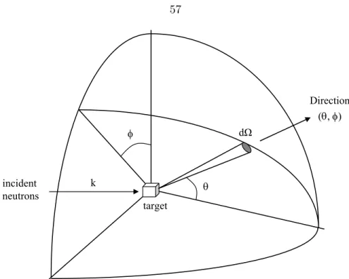
3.2.2 Theory . . . 56
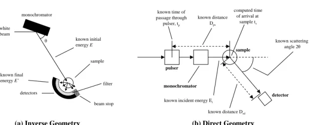
3.2.3 Indirect geometry spectrometers . . . 60
3.2.4 Direct geometry spectrometers . . . 61
4 Hydrogen adsorption by graphite intercalation compounds 62 4.1 Introduction . . . 62
4.2 Hydrogen adsorption isotherms of KC24 . . . 63
4.3 Hydrogen adsorption isotherms of RbC24 and CsC24 . . . 66
4.4 Hydrogen adsorption kinetics . . . 69
4.5 Discussion . . . 70
4.6 Conclusion . . . 71
5 Hydrogen diffusion in potassium-intercalated graphite 73 5.1 Introduction . . . 73
5.2 Quasielastic neutron scattering . . . 74
5.2.1 Description . . . 74
5.2.2 Continuous diffusion . . . 74
5.2.3 Jump diffusion . . . 75
5.2.4 Concentration effects . . . 77
5.3 Experimental methods . . . 78
5.4 Quasielastic scattering results . . . 79
5.5 Honeycomb lattice diffusion model . . . 80
5.6 Estimates of diffusion coefficients . . . 90
5.6.1 Low-Qlimit . . . 90
5.6.2 High-Qlimit . . . 92
5.6.3 Distribution of jump frequencies . . . 94
5.7 Measurements at longer timescales . . . 97
5.7.1 Overview . . . 97
5.7.2 Methods . . . 97
5.7.3 Quasielastic scattering . . . 98
5.7.4 Elastic intensity . . . 98
5.8 Molecular dynamics simulations . . . 101
5.8.1 Computational details . . . 101
5.8.2 Results . . . 103
5.8.3 Concentration effects . . . 106
5.9 Discussion . . . 109
5.9.1 Comparison with carbons, zeolites, and MOFs . . . 109
5.9.2 Diffusion on two time-scales . . . 110
5.9.3 Phase transformations . . . 111
5.10 Conclusions . . . 113
6.1 Introduction . . . 114
6.2 Background . . . 115
6.2.1 Rotational energy levels of the free hydrogen molecule . . . 115
6.2.2 Ortho- and para-hydrogen . . . 115
6.2.3 One-dimensional hindered diatomic rotor . . . 116
6.2.4 Scattering law for rotational transitions of molecular hydrogen . . . 118
6.3 Experimental methods . . . 120
6.4 Results . . . 124
6.4.1 Low-energy IINS spectra . . . 124
6.4.2 Diffraction pattern from low-energy IINS spectra . . . 125
6.4.3 Intermediate and high-energy IINS spectra . . . 126
6.4.4 IINS spectra of HD and D2 adsorbed in KC24 . . . 128
6.5 Hydrogen bound states studied by DFT . . . 133
6.5.1 Computational details . . . 133
6.5.2 Results . . . 134
6.6 Discussion . . . 142
6.7 Conclusion . . . 145
7 Conclusions 147 7.1 Summary . . . 147
7.2 Future work . . . 149
7.2.1 Thermodynamic trends . . . 149
7.2.2 Two-dimensional diffusion . . . 150
7.2.3 Translational-rotational coupling . . . 150
A Effect of porous texture on hydrogen adsorption in activated carbons 151 A.1 Introduction . . . 151
A.2 Experimental Methods . . . 153
A.3 Results . . . 155
A.4 Discussion . . . 161
A.5 Conclusion . . . 163
B Hydrogen absorption behavior of the ScH2-LiBH4 system 164 B.1 Introduction . . . 164
B.2 Experimental Details . . . 166
B.3 Results . . . 168
B.4 Discussion . . . 174
B.5 Conclusion . . . 175
Bibliography 177
List of Figures
1.1 Phase diagram of molecular hydrogen . . . 2
1.2 Optimizing the adsorption enthalpy with the Langmuir model . . . 6
1.3 Illustration of dispersion interactions between two semi-infinite slabs . . . 8
1.4 Structure of a hydrogen monolayer on graphene . . . 14
1.5 Structures of MOF-5, zeolite A, and activated carbon . . . 17
1.6 Maximum hydrogen adsorption capacities of various porous adsorbents plotted against their BET surface area . . . 19
2.1 Isobars of the potassium-graphite system . . . 23
2.2 Structure of the KC24 compound . . . 24
2.3 Possible in-plane structures of the KC24 compound . . . 27
2.4 Domain model for the CsC24 compound . . . 28
2.5 Synthesized samples of KC24 . . . 31
2.6 Powder XRD pattern of synthesized KC24sample . . . 32
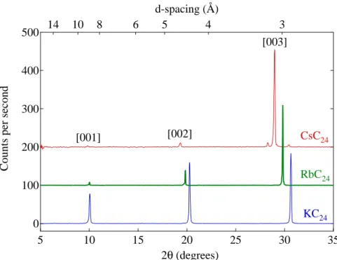
2.7 Comparison of the powder XRD patterns from stage-1, stage-2, and stage-3 potassium graphite intercalation compounds . . . 33
2.8 Comparison of of KC24, RbC24, and CsC24 . . . 33
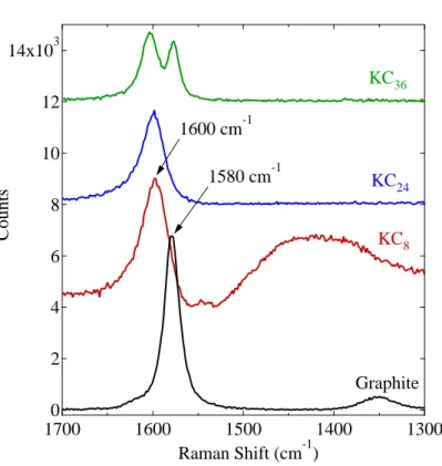
2.9 Raman spectra of potassium graphite intercalation compounds . . . 35
2.10 Neutron diffraction patterns for a deuterated KC24powder . . . 37
2.11 Pair distribution function of deuterated KC24at 35 K . . . 38
3.1 Illustration of surface excess adsorption . . . 41
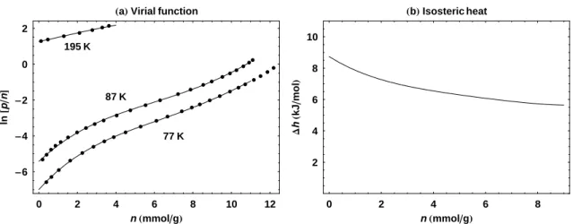
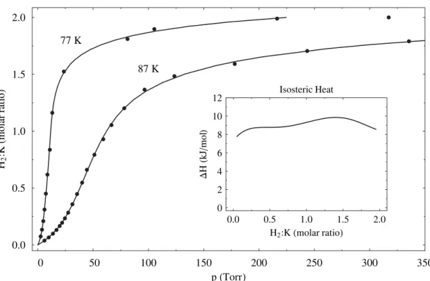
3.2 Isosteric heat from fitting empirical functions separately to each isotherm . . 45
3.3 Isosteric heat from fitting to a single virial-type thermal equation . . . 46
3.4 Differential enthalpy of adsorption in the Henry’s law regime . . . 48
3.5 Schematic illustration of the Sieverts instrument. . . 50
3.6 Correcting for empty reactor adsorption . . . 54
3.7 Wavevectors and position vectors for a neutron scattering event . . . 56
3.8 Typical geometry of a neutron scattering experiment . . . 57
3.9 Schematic illustration of an inverse geometry neutron spectrometer and a di- rect geometry spectrometer . . . 60
4.1 Hydrogen adsorption isotherms of a flake-graphite KC24 sample . . . 63
4.2 Virial-type thermal equation fitted to the KC24 isotherm . . . 64
4.3 Adsorption isotherms of a Grafoil-based KC24 sample . . . 65
4.4 Hydrogen adsorption isotherms of an RbC24 sample . . . 67
4.5 Hydrogen adsorption isotherms of an CsC24 sample . . . 68
4.6 Hydrogen adsorption enthalpies for KC24, RbC24 and CsC24 . . . 68
4.7 Kinetics of hydrogen adsorption by RbC24. . . 69
5.1 Scattering law for continuous 2D diffusion . . . 76
5.2 QENS spectra of KC24(H2)0.5 between 80 K and 110 K . . . 80
5.3 Hydrogen sublattice on KC24 . . . 81
5.4 Linewidth of the honeycomb net model function plotted versus momentum transfer . . . 84
5.6 QENS spectra at 90 K fitted to the honeycomb net jump diffusion model . . 87
5.7 QENS spectra at 100 K fitted to the honeycomb net jump diffusion model . . 88
5.8 QENS spectra at 110 K fitted to the honeycomb net jump diffusion model . . 89
5.9 Experimental KC24(H2)0.5 spectra at 110 K fitted to the two-dimensional con- tinuous diffusion model . . . 91
5.10 The five largest momentum-transfer groups of the 110 K data . . . 93
5.11 The QENS spectra of KC24(H2)0.5 fitted to the FT-KWW function . . . 95
5.12 Fit parameters for the FT-KWW function . . . 96
5.13 Comparison of QENS spectra measured on DCS and HFBS spectrometers . . 99
5.14 Elastic intensity scan of KC24(H2)1 and KC24(H2)2 . . . 100
5.15 Molecular dynamics trajectories of KC28(H2)1 . . . 102
5.16 Mean square displacement from MD simulations at 70 K . . . 104
5.17 Comparison of experimental and simulated hydrogen diffusion coefficients in KC24(H2)1 . . . 106
5.18 Intermediate scattering functions calculated from MD trajectories . . . 107
5.19 Effect of H2 composition on QENS spectra of CsC24 at 65 K . . . 108
5.20 Hydrogen diffusivity in various adsorbents compared to KC24 . . . 109
6.1 Rotational energy level transitions for 1D hindered rotor model . . . 117
6.2 Molecular form factors for pure rotational transitions of the H2 molecule . . 118
6.3 Low-energy-transfer IINS spectra of KC24(H2)x . . . 122
6.4 Decomposition of the low-energy-transfer IINS spectra of KC24(H2)x into a sum of Gaussian curves . . . 123
6.5 Diffraction pattern of KC24(H2)x measured on DCS at 4 K. . . 125
6.6 Intermediate-energy IINS spectra of KC24(pH2)x . . . 127
6.7 High-energy IINS spectra of KC24(pH2)x . . . 129
6.8 Intermediate-energy IINS spectra of D2, HD, and p-H2 adsorbed in KC24 . . 131
6.9 Comparison of the IINS spectra from p-H2, HD, and D2 . . . 132
6.10 Calculated potential energy surface for the KC28 unit cell . . . 135
6.11 One-dimensional slices through the potential energy surface . . . 137
6.12 Line scans for different H2 orientations . . . 138
6.13 Orientational potential of H2 in the theoretical KC28 structure . . . 139
6.14 Transition energies for the anisotropic hindered rotor model . . . 141
A.1 Surface texture analysis for the ACF-10 sample . . . 154
A.2 High-resolution TEM image of the ACF-10 sample . . . 156
A.3 Pore size distributions of the ACF-10, ACF-20, and CNS-201 samples, as determined by the DFT method . . . 158
A.4 Hydrogen adsorption isotherms of ACF-10, ACF-20, and CNS-201 . . . 159
A.5 Isosteric heats measured for ACF-10, ACF-20, and CNS-201 . . . 161
B.1 Synthesis of scandium hydride . . . 167
B.2 Kinetic desorption data for the ScH2+ 2 LiBH4 system . . . 169
B.3 Powder X-ray diffraction patterns for the ScH2+ 2 LiBH4 system . . . 171
B.4 NMR spectra of milled and dehydrogenated ScH2+ 2 LiBH4 . . . 172
B.5 Comparison of the Raman spectra of dehydrogenated ScH2+2 LiBH4 and neat LiBH4 . . . 173
List of Tables
1.1 Current DOE revised technical targets for on-board hydrogen storage systems
for light-duty vehicles . . . 3
1.2 Major hydrogen storage methods . . . 4
2.1 Lattice parameters of K, Rb, and Cs graphite intercalation compounds . . . 34
3.1 Important definitions for adsorption . . . 41
4.1 Hydrogen adsorption by KC24, RbC24, and CsC24 . . . 66
5.1 Fit parameters for the honeycomb net jump diffusion model . . . 90
5.2 Self-diffusion coefficients of KC24(H2)0.5 determined from QENS . . . 92
5.3 Jump diffusion residence times of KC24(H2)1 measured on the DCS and HFBS spectrometers . . . 99
6.1 Summary of peak positions and peak areas of the low-energy IINS spectra . . 124
6.2 Summary of peak positions and peak areas of the intermediate and high-energy IINS spectra . . . 129
6.3 Comparison of peak positions of the intermediate IINS spectra for p-H2, HD, and D2 adsorbed in KC24 . . . 132
6.4 Transition energies predicted by the one-dimensional hindered rotor model for various barrier heights . . . 143
A.1 Surface texture parameters for ACF-10, ACF-20, and CNS-201 . . . 157 A.2 Hydrogen adsorption parameters for ACF-10, ACF-20, and CNS-201 . . . 160
Chapter 1
Hydrogen Storage Materials
1.1 Introduction
Hydrogen has drawn attention as a next-generation energy carrier for mobile and station- ary power sources [1]. It has a number of advantages over other chemical energy carriers.
First, the energy conversion process is a clean one, with water as the waste product. Sec- ond, hydrogen can be produced reversibly by the dissociation of water. Lastly, hydrogen has a large chemical energy density per mass of around 39 kWhkg−1, about three times larger than that of chemical fuels such as liquid carbons [2]. For applications with fuel cell vehicles, hydrogen needs to be stored at high densities . Ideally, it should be contained within a small volume without adding too much additional weight to the vehicle. A driving range of at least 300 miles is considered crucial for the commercial success of a light-duty vehicle. This translates into an on-board storage requirement of 5 kg to 13 kg of hydrogen based on projected future fuel cell efficiencies [3]. Unlike other chemical fuels, however, the intermolecular forces in hydrogen are very weak. At ambient conditions of 20°C and 1 bar, a mass of 1 kg of hydrogen occupies a volume of 11.9 m3. The goal of hydrogen storage research is to decrease this volume while staying within specific temperature and pressure limits.
5 kg/m³ 15 kg/m³ 25 kg/m³ 35 kg/m³
45 kg/m³ 55 kg/m³
65 kg/m³ 75 kg/m³
85 kg/m³
solid liquid gas
triple point
critical point
10.0 100.
0.100 1.00 10.0 100.
1000.
Temperature (K)
Pressure (bar)
5 kg/m³ 15 kg/m³ 25 kg/m³ 35 kg/m³
45 kg/m³ 55 kg/m³
65 kg/m³ 75 kg/m³
85 kg/m³
solid liquid gas
triple point
critical point
10.0 100.
0.100 1.00 10.0 100.
1000.
Temperature (K)
Pressure (bar)
5 kg/m³ 15 kg/m³ 25 kg/m³ 35 kg/m³
45 kg/m³ 55 kg/m³
65 kg/m³ 75 kg/m³
85 kg/m³
solid liquid gas
triple point
critical point
15: Pressure vs. Temperature plot: hydrogen (normal)
Figure 1.1: Phase diagram for H2. The melting line and the liquid-vapor line are drawn as bold lines. The triple point and the critical point are both labeled. Constant density contours are drawn as thin lines.
1.2 Physical storage of hydrogen
The fundamental difficulty of storing hydrogen as a liquid or compressed gas is evident in the hydrogenp-T phase diagram shown in Fig. 1.1. At the triple point (T = 13.803 K,p= 0.0704 bar) the solid density is ρs = 86.48 kg m−3, the liquid density is ρl = 77.03 kg m−3, and the vapor pressure is a modest 0.07 bar. In the small region between the triple point and the critical point, hydrogen exists as a liquid with a normal boiling point of 20.39 K.
If liquid hydrogen is stored in a closed vessel, continuous boil-off can lead to pressures of 104bar. The critical point (Tc = 32.98 K, pc = 13.25 bar) of H2 occurs at a temperature
light-duty vehicles
Storage Parameter Units 2010 2015 Ultimate
System gravimetric capacitya kg(H2)/kg(System)b 0.045 0.055 0.075
kWh/kg (1.5) (1.8) (2.5)
System volumetric capacity kg/m3 28 40 70
kWh/m3 (900) (1300) (2300)
Min/max delivery temperature K 233/358 233/358 233/358
Cycle life Cycles 1000 1500 1500
Min delivery pressure atm 4FC/35ICEc 3FC/35ICE 3FC/35ICE
Max delivery pressure atm 100 100 100
System fill time kg/min 1.2 1.5 2.0
Fuel purity Percent H2 99.99 (dry basis)
aThe listed gravimetric and volumetric capacities aresystem targets that include the mass and volume of the system itself, including the tank, material, valves, regulators and other parts.
Material capacities may need to be up to twice as large as system capacities. See Ref. [4].
bThe standard practice here is to define the gravimetric (volumetric) density relative to the maximum final mass (volume) of the combined hydrogen-host system.
cFC=fuel cell, ICE=internal combustion engine
which is quite low compared to other gases. Above this temperature hydrogen cannot be liquefied by increasing the pressure. Therefore if the storage system is to operate at higher temperatures, the hydrogen will exist in the gas phase. From the constant density contours in Fig. 1.1, it is clear that at room temperature a pressure of over 1000 bar is required to achieve densities on the order of the liquid or solid phases. This is possible using carbon- fiber-reinforced high-pressure cylinders, but is undesirable for on-board vehicle storage.
1.3 Technical targets for hydrogen storage materials
The U.S. Department of Energy’s 2010 and 2015 technical targets for on-board vehicu- lar hydrogen storage are a useful benchmark for comparing different storage methods [4].
Several of the current DOE technical targets are listed in Table 1.1. Operational charac- teristics such as the temperature, the min/max delivery pressure, the re-filling time, the cycle life, and the fuel purity are also crucial to the performance of the storage system.
Table 1.2: Comparison of hydrogen storage methods
Method ρm(wt%)a ρv(kg m−3)b T (K)c p(bar)d Description Compressed
gas
13 <40 273 800 Compressed hydrogen gas;
lightweight, high-pressure cylinder
Liquid Varies 70.8 21.5 1 Liquid hydrogen, continuous loss
of a few % per day at RT
Physisorption ≈2 20 77 100 Physical adsorption by porous
materials, fully reversible Interstitial
metal hydrides
≈2 150 273 1 Atomic hydrogen occupies
interstitial sites, fully reversible, metals are heavy
Complex hydrides
<18 150 >100 1 Complex compounds [BH4]– or [AlH4]–, desorption at elevated temperature, adsorption at high pressure
Chemical hydrides
<40 >150 273 1 Thermal decomposition of chemical hydrides, not directly reversible
aGravimetric storage density bVolumetry storage density cOperational temperatures for storage method
dOperational pressures for the storage method eTable adapted from Ref. [2]
It is these criteria that make physical adsorption (i.e., physisorption) an attractive storage method. Adsorbed hydrogen does not chemically react during adsorption and, therefore, does not accumulate impurities which can poison the fuel-cell downstream. Because it does not involve bulk solid diffusion or chemical dissociation, the physisorption process is also extremely fast and fully reversible, allowing it to meet both the cycle-life and refilling-time targets. In Table. 1.2, physisorption is compared to the five other basic storage methods.
The fundamental problem with physisorption-based storage is that, due to the weak bind- ing interaction between the H2 and the adsorbent surface, the hydrogen density at ambient conditions is too small.
1.4 Storage based on physisorption
Physical adsorption is a process where gas admolecules bind weakly onto the adsorbent surface by van der Waals (vdW) forces. Chemical bonds are not formed. The equilibrium
and the strength of the surface interaction. The adsorbed layer and the bulk gas are in equilibrium so the Gibbs free energies must be equal: Ggas=Gads. SubstitutingG=H−T S yields
Hads−Hgas=T(Sads−Sgas). (1.1)
Adsorption involves a reduction in the degrees of freedom of the gas molecules so a tentative assumptionSgasSads can be made. For many adsorbents a change in entropy of−8Rcan be estimated [5]. A simple estimate of the required enthalpy for room temperature storage is
∆H =Hads−Hgas≈ −8RTroom=−20 kJ mol−1. (1.2)
The importance of adsorption thermodynamics can be better illustrated using the Langmuir model.1 For an equilibrium pressure p, the amount of adsorbed gas is given by
n(p) =nmax
Kp 1 +Kp
, (1.3)
wherenmax is the maximum adsorption capacity of the material, andK is the equilibrium constant (which depends on both the temperature and the change in Gibbs free energy).
As indicated in Table 1.1, hydrogen should be delivered between a minimum pressure of pmin = 3 bar and a maximum pressure of pmax = 100 bar. The storage system cycles between these operational pressure limits, and the total delivered hydrogen is the difference between n(pmax) and n(pmin). We want to determine the enthalpy which optimizes the hydrogen delivery between these pressure limits [5]. For an operating temperature of 298 K,
1Although the Langmuir model is meant to describe non-interacting adsorbed monolayers on a homoge- neous surface, it also works well for describing hydrogen adsorption in microporous materials [6].
1.0
0.8
0.6
0.4
0.2
0.0 n / nmax
100 80
60 40
20 0
Pressure (bar)
∆n-18 kJ/mol
∆n-6 kJ/mol
3 bar 100 bar
∆n-25 kJ/mol
∆H = -25 kJ/mol ∆H = -18 kJ/mol ∆H = - 6 kJ/mol
∆n — Hydrogen delivery between 3 bar and 100 bar
Figure 1.2: Langmuir isotherms for three different adsorption enthalpies (∆H). Hydrogen delivery (∆n) for each isotherm is indicated by the vertical distance between the adsorption amounts at 3 bar and 100 bar.
realistic estimates of the optimum adsorption enthalpy typically give values around ∆H=
−18 kJ mol−1 [7]. In Fig. 1.2, Langmuir adsorption isotherms are illustrated for various enthalpies of adsorption. It can be seen that the hydrogen delivery depends very strongly on the enthalpy. Because the isotherm for ∆H =−25 kJ mol−1 is very steep, for example, most hydrogen remains adsorbed when the pressure cycles down to 3 bar. On the other hand, the−6 kJ mol−1 isotherm is very low, containing only a small amount of adsorbed hydrogen at 100 bar. An optimal adsorption enthalpy would occur between these two extremes, providing a larger amount of deliverable hydrogen capacity.
This example demonstrates the importance of adsorption enthalpy in determining the properties of a physisorption-based storage system. Because heterogeneous adsorption sites and hydrogen-hydrogen lateral interactions are omitted from the model, the adsorption
that decreases as a function of n, then hydrogen delivery is typically reduced [5]. This makes sense because a single enthalpy can be better optimized than a varying one simply by choosing the optimum enthalpy for every adsorption site. The ideal adsorbent for an isothermal storage system will likely have a constant ∆H of around−18 kJ mol−1, although the specific values will depend on the operational pressure and temperature ranges.
1.5 The mechanism of physisorption
1.5.1 Overview
In Section 1.4 it was illustrated that the enthalpy of adsorption plays a central role in the operational characteristics of a physisorption-based system. To determine the thermody- namic limits of such a storage system a detailed understanding of this interaction energy is critical. Unfortunately, ab initio modeling of physisorption is much less developed than it is for chemisorption. The reason is that dispersion forces play a large role in the ph- ysisorption mechanism. Although density functional theory works quite well for chemically bound systems, it does not accurately treat long-range interactions of weakly-bound sys- tems [8]. First principles methods capable of treating dispersion forces include the MP2 method (second-order Møller-Plesset perturbation theory) and CCSD(T) method (coupled cluster with single, double, and triple excitations). However these methods are too compu- tationally expensive to apply to realistic adsorbent systems. In fact, empirical potentials are still a starting point for many computational studies of physisorption. In this section, the three main types of hydrogen physisorption interactions will be described.
A B ε
Aε
0= 1 ε
BVacuum
l
Figure 1.3: Schematic drawing of two semi-infinite slabs of material A and material B with a separation length ofl. The region between the two slabs is vacuum. The dielectric constants of the three regions are denotedA,B and0. Adapted from Ref. [9].
1.5.2 Dispersion interactions2
A famous example of dispersion forces is provided by the interactions between electrically neutral gas particles which cause deviations from ideal gas behavior at high densities. In brief, dispersion interactions are weak, long-range, nonspecific interactions which are due to charge fluctuations in the two interacting materials. These fluctuations can be due to phenomena such as ionic movements, dipole rotations, and dipole vibrations at the lower frequency end. However, it is the higher frequency electron fluctuations caused by the quantum mechanical uncertainty in position and momentum which contribute most to the interaction. A simple macroscopic system of dispersion interactions between material A and material B across a region of vacuum is illustrated in Fig. 1.3. An electron fluctuating in material A emits an oscillating electric field across the vacuum into material B. This in turn enhances charge fluctuations in material B which lower the overall electromagnetic energy. The mutual fluctuations in material A and material B are not simply random, but have a correlation that affects the total energy and results in a net force. The susceptibility
2The analysis presented in this section closely follows Ref. [9].
itself depends on the frequency of the oscillations. The free energy per unit area required to bring slabs A and B from infinity to a separationl is given by the Hamaker equation,
G(l) = kBT 8πl2
∞
X
n=0
dA(ξn)dB(ξn)Rn(l), (1.4)
where the relative difference between the material dielectric responsesA(ξ) andB(ξ) and the vacuum dielectric response 0 = 1 is given by
dA(ξ) = A(ξ)−1
A(ξ) + 1, dB(ξ) =B(ξ)−1
B(ξ) + 1. (1.5)
The relativistic screening term,Rn(l), damps the electron correlations at large distances due to the finite time that the fluctuating electric fields take to reach the other material. Since Rn(l) is only important at large separation distances, it can be ignored for physisorption.
The sum in Eq. 1.4 is taken over a discrete sampling of the frequency (ξn).3 The lowest frequencies are on the order of the thermal energy and may originate from vibrations or rotations of polar molecules. However, the sum is dominated by the larger UV and X-ray frequency range.
This macroscopic analysis can be reduced to the familiar point-particle interaction for- mulas if we assume material A and material B are regions of a dilute gas. In this case = 1 +N α, where N gives the number density of the dilute gas. The total polarizability
3The variableξ is the imaginary component of the complex frequency, ω=ωR+iξ. Another way to write this is exp (iωt) = exp (−ξt) exp (iωRt). The real frequency,ωR, corresponds to sinusoidal behavior, while the imaginary frequency represents a decaying exponential. The dielectric responses are expressed in terms of a characteristic relaxation time (τ) over which a spontaneous charge fluctuation dies out. For example, the UV and X-ray regions have relaxation times on the order of τ ≤ 10−17sec while molecular vibrations have τ ≤10−16sec. When written in terms of the relaxation time, the dielectric response is a smoothly varying curve. This is preferable to the large spikes near resonance that occur when the dielectric response is expressed in terms ofωR.
α of each gas molecule consists of the permanent dipole moment (µdip) and the inducible polarizability (αind). If the molecules have a permanent dipole moment, then dipole-dipole (Keesom) and dipole-induced-dipole (Debye) interactions are present. These are the “zero- frequency” electrostatic interactions, given by
(Keesom) g(r) =− µ4dipole
3kBT r6, (1.6a)
(Debye) g(r) =−2µ2dipole
r6 αind(0). (1.6b)
The London force is caused by electron correlations at all frequencies. When the retardation screening factor is omitted, this interaction reads as
(London) g(r) =−6kBT r6
∞
X
n=0
α2ind(iξn). (1.7)
London originally derived the r−6 expression in 1930 for two hydrogen atoms at large separation. From accurate first-principles calculations it is known that when hydrogen interacts with large molecules, the energy minimum for the London force occurs at about one molecular radius and has a binding energy on the order of several kJ mol−1 [10]. When the charge distributions overlap at small separations, Pauli repulsion becomes the dominant force; it is typically modeled with a repulsiver−12component in a Lennard-Jones potential.
1.5.3 Electrostatic interactions
The hydrogen molecule does not have a permanent dipole moment. Due to the prolate, non- spherical shape of the H2 molecule, the first non-zero multipole moment is the quadrupole moment. The ion-quadrupole interaction goes asr−3 as a function of distance. Further, the hydrogen molecule is polarizable in the presence of external fields, and the ion-induced-
teracting with a unit charge at a distance of 3 ˚A, the ion-quadrupole interaction energy is about 3.5 kJ mol−1 [10]. The associated ion-induced-dipole interaction energy is about 6.8 kJ mol−1[10]. In the presence of a strong external field, it would appear that electrostatic interactions are considerably larger than dispersion interactions. In reality, though, few ad- sorbent systems actually contain unscreened ionic charges. Even in a first approximation, dispersion forces cannot be ignored for physisorption systems.
1.5.4 Orbital interactions
Molecular hydrogen contains a ground state bonding orbital σg with an energy level of about −11.7 eV. There is a relatively large energy gap between the bonding orbital σg and the unoccupied anti-bonding orbital σu∗ with a magnitude of about 2 eV [10]. Interactions between filled molecular orbitals are primarily repulsive. However interactions between filled and unfilled orbitals can result in charge transfer, donor-acceptor bonding, and over- all stabilization. Orbital interactions have shorter bond lengths and larger binding energies than dispersion interactions. Charge transfer causes an elongation of the H2 bond length, which is directly measurable by a softening of the intramolecular vibrational modes. Transi- tion metals (TM) are known to form H2 coordination complexes (i.e., “Kubas” complexes) in which H2-σ to TM-d electron-transfer is coupled with TM-d to H2-σ∗ electron back- donation [11]. In reality, though, hydrogen does not easily donate or accept charge due to the large separation between its σg and σu∗ orbitals. In fact, the adsorption mechanism in many metal-organic frameworks with exposed transition metal sites can actually be ex- plained in terms of electrostatic interactions, without the need for orbital interactions [12].
1.6 Carbon adsorbents
1.6.1 Overview
Carbon adsorbents are attractive for physisorption storage systems due to their simplic- ity, light weight, and low manufacturing cost. Considerable work has been performed in this field, and at least two review articles are available which describe the status of hy- drogen storage in carbon materials [13, 14]. Non-carbon adsorbents which are of particular importance to the hydrogen storage field are described briefly in Sec. 1.6.5.
Nonporous amorphous carbons can be thought of as agglomerates of spheroidal particles.
In this case the specific surface area (SSA) consists of the external particle areas, typically in the range of 2 m2g−1 to 200 m2g−1, depending on the particle size. A porous material contains narrow internal cavities or channels which connect to the particle surface. Pore sizes are classified by IUPAC as micropores (pore width < 2 nm), mesopores (pore width 2–50 nm) and macropores (pore width>50 nm) [6]. Microporous carbons are of particular importance for hydrogen storage since they contain large surface areas and provide strong binding sites.
1.6.2 Graphite
Graphite is an ordered carbon allotrope consisting of alternating layers of sp2 bonded trig- onal planer sheets. Neighboring planes interact by overlapping π-bonds between the un- hybridized carbon 2p orbitals. The stacking sequence of the basal planes along the c-axis follows a staggered -ABAB- pattern, so that half of the carbon atoms in a given plane sit between the hexagon centers of the layers above and below it.4 The carbon-carbon bond
4Rhombohedral graphite follows an -ABCABC- stacking sequence.
Graphitic carbons are nonporous, with surface areas typically under 20 m2g−1, and negligibly small hydrogen uptake at low temperature [6]. The measured adsorption enthalpy of hydrogen on Graphon6 is 3.8 kJ mol−1 [15], well below the targeted value. One strategy for increasing the binding energy for carbon adsorbents is to open up space between the layer planes in order to accommodate guest molecules. In fact, this hypothetical graphene slit-pore structure has been the subject of numerous computational studies [16–18]. Due to the overlapping potential fields from opposing slit-pore walls, the heat of adsorption is enhanced. The optimal interlayer spacing would be large enough to accommodate two hydrogen monolayers (i.e., one monolayer per slit pore wall). Any additional interlayer expansion would not be useful because hydrogen only adsorbs in monolayers at supercritical temperatures.
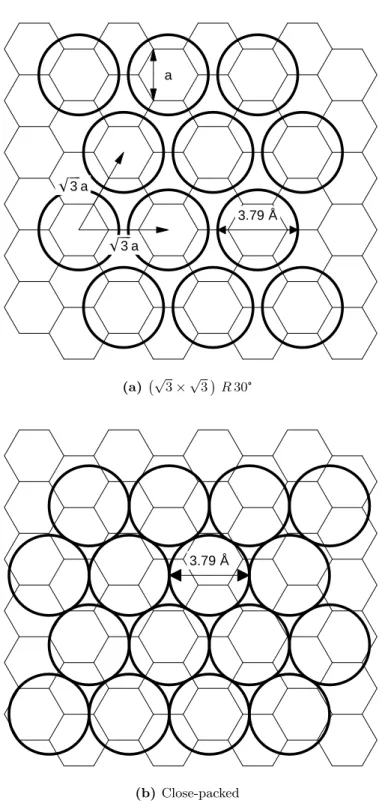
Although the graphene slit pore structure is well-suited for optimizing the carbon- hydrogen binding interaction, the general consensus is that the gravimetric density is in- trinsically low due to the geometry. This can be illustrated by considering H2 monolayers on an ideal graphene sheet. An estimate of the graphene specific surface area is obtained from the fact that a single hexagon contains a net total of two carbon atoms with an area of 1.5√
3a2. This gives an SSA of 2633 m2g−1 on double-sided graphene. Two possible configurations for a hydrogen monolayer on a graphene surface are illustrated in Figure 1.4.
Commensurate structures are energetically favorable since the hydrogens sit in the hexagon centers, but they have a lower density than a close-packed structure. If both sides of the graphene surface are occupied, then the gravimetric density is 5.6 wt% for the commensurate
5This structure corresponds to an ideal graphite crystal, whereas natural graphite contains both hexag- onal and rhombohedral modifications, as well as large deviations from the ideal stacking sequence. Natural graphite also contains large amounts of chemical impurities.
6Graphon is a graphitized carbon black material with a surface area of 90 m2g−1 which is typically used as a substitute for graphite in adsorption measurements
3.79 Å
!!!!3 a
!!!!3 a
a
(a) √ 3×√
3 R30°
3.79 Å
(b)Close-packed
Figure 1.4: Two possible structures for a hydrogen monolayer on a graphene sheet.
be obtained by using the standard method of estimating the BET cross-sectional area [6].
For a hexagonal close-packed structure, the cross-sectional area of a hydrogen molecule is given by
σ=f M
ρNa
2/3
, (1.8)
where the HCP packing factorf is 1.091,ρis the density of liquid hydrogen,M is the molar mass, and Na is Avogadro’s number. Taking the solid H2 density as ρ= 86.48 kg m−3, the cross-sectional area is σ = 0.124 nm2. If the carbon specific surface area is a(SSA), then the hydrogen monolayer adsorption in wt% is
wt% =
a(SSA) σ
M Na
×100. (1.9)
This gives 1.34 wt% per 500 m2g−1 carbon surface area. Double-sided graphene has a surface area ofa(SSA) = 2633 m2g−1, which translates to a maximum hydrogen adsorption of 7.04 wt%. This represents the theoretical limit for H2 density in a pillared graphene structure.
1.6.3 Fullerenes
Another strategy to enhance hydrogen binding in carbon adsorbents is to use a curved carbon surface. Fullerenes, such as single-walled carbon nanotubes (SWCN) and C60 buck- eyballs, are well-known examples. They are formed from graphene-like sheets composed of five or six-member rings. The presence of pentagonal rings results in the curvature of the carbon planes, allowing the formation of C60 spheres. Similarly, the hollow cylindrical
7We can adopt the nearest-neighbor distance of solid hydrogen (3.79 ˚A) as a conservative estimate of the hard sphere diameter.
structure of single- and multi-wall carbon nanotubes is obtained by rolling up graphene sheets along different directions. Unfortunately, a large amount of variation and irrepro- ducibility has plagued both experimental and theoretical work on hydrogen adsorption in fullerenes. Recent studies have indicated that carbon nanotubes have the same adsorption properties as activated carbons and other amorphous carbons [19, 20]. Nevertheless, as the only ordered allotropes of carbon that adsorb hydrogen, fullerenes provide a unique plat- form for rigorously studying the hydrogen-carbon interaction from both an experimental and theoretical level. For example, the diameter of the SWCNs is a tunable parameter which can be used to optimize the adsorption behavior.
1.6.4 Activated Carbons
Activated carbons are predominantly amorphous materials with large surface areas and pore volumes, often containing BET areas in excess of 2000 m2g−1. They are best described as “a twisted network of defective carbon layer planes cross-linked by aliphatic bridging groups [21].” The pore structure of an activated carbon is complex and ill-defined, making it challenging to study. An example of this complex, cross-linked structure is illustrated in Fig. 1.5c. Activated carbons are produced in industrial quantities from a carbon-rich pre- cursor by a physical or chemical activation process. Physically activated carbons commonly use bituminous coal or coconut shells as a starting material. The two-stage activation pro- cess consists of carbonization, where oxygen and hydrogen are burned off, and gasification where the char is heated in a steam or carbon dioxide atmosphere to create a highly porous structure from carbon burn-off. Carbon aerogels are a separate class of amorphous car- bons which can mimic the properties of activated carbons. They are prepared by a sol-gel polymerization process and can be activated using the standard methods.
(a)MOF-5 (b)Zeolite A (c) Activated carbon
Figure 1.5: Structure of (a) MOF-5, (b) zeolite A, and (c) activated carbon.
1.6.5 Zeolites
Zeolites are crystalline materials composed of SiO4 or AlO4 building blocks. They contain an intra-crystalline system of channels and cages which can trap guest H2 molecules. The adsorption capacity of zeolites at 77 K is typically below 2 wt%. A theoretical capacity of 2.86 wt% has been suggested as being an intrinsic geometric constraint of zeolites [22].
Due to this low gravimetric density, zeolites are not typically considered feasible hydrogen storage materials. Isosteric heats on the order of 6–7 kJ mol−1 are typical for hydrogen- zeolite systems [23]. Zeolite structures such as LTA (see Fig. 1.5b) can have intra-crystalline cavities on the order of the H2 diameter itself. They function as molecular sieves, blocking adsorption of larger gas molecules by steric barriers. They also exhibit quantum sieving effects on hydrogen isotopes. When confined inside a molecular-sized cavity, the heavier D2 molecule is adsorbed preferentially over the lighter H2 molecule due to its smaller zero-point motion [24].
1.6.6 Metal-organic frameworks
Metal-organic frameworks (MOFs) are synthetic crystalline materials which are somewhat analogous to zeolites. Organic linker molecules form the building blocks of MOFs, coordina-
tively binding to inorganic clusters to form a porous framework structure. A good example of a MOF structure is provided by MOF-5, which consists of Zn4O(CO2)6 units connected by benzene linkers in a simple cubic fashion (Fig. 1.5a). It was not until fairly recently that MOFs were studied as a potential hydrogen storage material [25]. By modifying the organic linkers, the pore size and effective surface area can be tailored quite effectively. Hydrogen adsorption capacities of up to 7.5 wt% at 77 K have been measured for MOF-177 [26, 27].
A number of MOFs contain coordinatively unsaturated metal centers which are known to enhance hydrogen binding interactions [28]. In most cases this interaction is dominated by electrostatic contributions [12, 29, 30], but the possibility of stronger “Kubas” orbital interactions between the hydrogen and the open metal sites has generated considerable interest.
1.6.7 Hydrogen adsorption by porous carbons
Hydrogen adsorption at supercritical temperatures is characterized by weak interactions between the adsorbed hydrogens. Interactions between the hydrogen and the adsorbent surface are dominant, favoring the formation of adsorbate monolayers. Multilayer formation has a characteristic energy on the order of the hydrogen heat of condensation (0.9 kJ mol−1) and does not occur above the critical temperature. Capillary condensation of H2 inside large pores or cavities is not possible, resulting in a reduction of the usable pore volume.
Therefore, micropores are the most important feature of an adsorbent while mesopores contribute little to the total hydrogen capacity.
Many studies have noted a roughly linear relationship between the BET surface area and the maximum H2adsorption capacity at 77 K [20,31]. The simple rule-of-thumb for this behavior is 1 wt% per 500 m2g−1. This can be compared to the 1.34 wt% per 500 m2g−1
5
4
3
2
1
0 H2 Capactity at 77 K (wt%)
3000 2500
2000 1500
1000 500
0
Specific Surface Area ( m2/g) MOF74
As-prepared aerogel Aerogel 850 °C Aerogel 1050 °C Activated aerogels ACF-1603 CNS-201 Close-packed H2
1 wt% per 500 m2/g
Figure 1.6: Maximum hydrogen adsorption capacities at 77 K of various adsorbents plotted against their BET specific surface areas. Materials include a series of carbon aerogels, two activated car- bon fibers (ACF-1603), one activated coconut carbon (CNS-201) and one metal-organic-framework (MOF-74). Straight lines indicate scaling between the specific surface area and storage capacity for close-packed hydrogen and for the rule-of-thumb (1 wt% per 500 m2g−1).
obtained for close-packed hydrogen on a double-sided graphene sheet. A sampling of data that was measured in our laboratory is summarized in Fig. 1.6. These samples included carbon aerogels (both activated and as-prepared), activated coconut-shell carbons, activated carbon fibers, and a metal-organic-framework (MOF-74). The scaling between hydrogen capacity and surface area is also plotted for both the empirical rule-of-thumb and the theoretical close-packed limit.
Surface areas do not always have a simple physical meaning for the complex disordered structure of activated carbons. What we should expect, however, is for a correlation to exist between the H2 uptake and the totalmicropore volume. Studies of both carbon and zeolite adsorbents have found that this type of correlation exists and is actually stronger than the correlation with total BET surface area [19, 32]. In fact, the pore volume obtained from
CO2 adsorption at 273 K is suggested as better reflecting the total micropore volume due to the faster admolecule diffusion. Hydrogen adsorption is therefore thought to be better correlated to the CO2 pore volume than to the standard N2 pore volume [32].
1.6.8 Chemically modified carbon adsorbents
There is a general consensus that carbon adsorbents will not meet density or operational targets for a hydrogen storage system at ambient temperatures [2, 33]. Maximum hydrogen capacity rarely exceeds 1 wt% at room temperature, even at pressures as high as 100 bar [34, 35]. This is an intrinsic property which is due to the low heat of adsorption. It applies equally to carbon nanostructures like SWCNs and to amorphous structures like activated carbons. The most promising strategy for increasing the adsorption enthalpy is through chemical modification of carbon adsorbents.
There are numerous computational studies of hydrogen uptake by hypothetical metal- doped carbon nanostructures. Decoration of C60buckeyballs with scandium [36] or titanium [37] is known to create strong binding sites for multiple H2 molecules. Metal-decorated SWCNs also exhibit enhanced hydrogen binding energies relative to the pristine material [38]. Computational studies of alkali metal doped graphene and pillared graphite structures have noted the importance of electrostatic effects in enhancing hydrogen binding [39, 40].
Experimental data exists for several metal-doped carbon adsorbents. Potassium-doped activated carbons show enhanced hydrogen adsorption at low pressures relative to the raw material, indicating a larger adsorption enthalpy [41]. Ball-milled mixtures of graphite and potassium adsorb modest amounts of hydrogen between 313 K and 523 K, but the adsorption is not reversible [42].
The understanding of the effect of chemical modifications on hydrogen adsorption is incom- plete. Numerous computational studies exist for hypothetical structures which are not easily synthesized. A large amount of experimental data exists for ill-defined structures such as activated carbons, which are difficult to model theoretically. Research on the fundamental thermodynamics of hydrogen adsorption remains important. In particular, a combination of experimental and computational data on the interaction of hydrogen with a well-defined, chemically-modified carbon adsorbent would provide much needed information. It was for this reason that I chose to study H2 adsorption in graphite intercalation compounds. This class of materials is introduced in the next chapter.
Chapter 2
Potassium Intercalated Graphite
2.1 Introduction
Graphite intercalation compounds (GICs) are a unique class of lamellar materials formed by the insertion of atomic or molecular guests between the layer planes of the host graphite.
Electrical, thermal and magnetic properties can be varied by intercalation, making these materials interesting technologically. Graphite intercalation compounds exist for all alkali metals, but only the K, Rb, and Cs compounds are known to adsorb hydrogen. The maximum adsorption capacity of these materials is only around 1 wt%, but their high degree of structural ordering makes them a model system for studying hydrogen adsorption in a carbon nanostructure. They share many similarities with a chemically-modified carbon slit-pore structure, and are readily synthesized. Due to the attractiveness of potassium as a lightweight dopant for carbon adsorbents, potassium intercalated graphite is the focus of this thesis.
2.2 History
Alkali metal GICs were first prepared by Fredenhagen and co-workers in the 1920’s with the compositions C8M and C16M [43]. Further studies were carried out on the potassium com-
12 10 8 6 4 2 0
K/C × 100
350 300
250 200
150 100
50 0
Tgraphite- Tpotassium (°C)
KC8
KC24 KC36
Figure 2.1: Composition of the potassium-graphite system based on the temperature difference between the graphite host and potassium vapor. Adapted from Ref. [44].
pound in the 1950’s by H´erold, who developed a two-zone, vapor-phase synthesis technique where the potassium melt was kept at a constant temperature (250°C) while the graphite temperature was varied (250°C to 600°C) [44]. Stoichiometric compounds of KC8 and KC24
are visible as plateaus in the potassium-graphite isobar illustrated in Fig. 2.1. Structural studies ofstaging in potassium GICs were performed by R¨udorff and Schulze [45]. Discrete compositions of MC8, MC24, and MC36were linked to the formation of stage 1, stage 2, and stage 3 intercalation compounds, respectively. The staging index, n, of the GIC indicates that the intercalant layer is found between everynth pair of host graphite planes. The stack- ing sequences in the alkali-metal GICs were further characterized by Perry and Nixon in the 1960’s [46]. In the early 1960’s, Saehr and H´erold discovered that KC8 chemisorbs hydrogen at elevated temperatures up to maximum values of about KC8H0.67 [47]. Chemisorption was also noted for RbC8 and KC24, but not for CsC8. Physisorption of H2 by the stage 2 compounds of K, Rb, and Cs at low temperatures was discovered by Tamaru and co-
(a) Side view (b)Top view
Figure 2.2: Structure of KC24. (a) The A|AB|BC|CA stacking sequence. (b) Possible in-plane potassium structure. Arrows from ABC describe the relative positions of the layer planes in the stacking sequence.
workers in the early 1970s [48]. These measurements were reproduced by a number of subsequent studies [49, 50]. The first inelastic neutron scattering studies of H2 adsorbed in the stage-2 alkali metals compounds were performed by White and co-workers in the early 1980’s [51]. Low-energy “rotational tunneling” peaks observed in the spectra indicated that the adsorbed hydrogen was in a strong anisotropic field. They were explained in terms of a one-dimensional hindered diatomic rotor model [52, 53]. By the late 1980’s, a substan- tial body of research existed on hydrogen-alkali-metal graphite intercalation systems (see Ref. [54] and [55] for reviews on this subject). Interest in the area dwindled during the 1990’s, as reflected in the small number of publications during the period. However with the emergence of hydrogen storage materials as a major topic of research, there has been a resurgence of interest in the hydrogen adsorption properties of the alkali-metal GICs.
2.3.1 Stacking sequence
Potassium GICs are formed by inserting potassium atoms into the galleries between the host graphitic layers. There are two competing forces in this system. First, the K atoms want to sit at the hexagon centers due to the strong graphite corrugation potential. This would cause the opposing basal planes to overlap exactly in an A|A sequence, where the vertical bar refers to the potassium layer. Second, the host graphite planes want to form a staggered sequence, ABAB, where half the carbon atoms in a given plane sit over the hexagon centers of the adjacent planes. It is the competition between these two driving forces that leads to the formation of discrete GIC stages. At low metal concentrations like KC24and KC36, it is apparently energetically favorable for metal layers to only occupy every 2ndand 3rdgraphite gallery, respectively. For this reason, KC24 and KC36 are called the stage-2 and stage- 3 compounds. The non-intercalated layers can maintain a staggered AB sequence, while the intercalated layers have an A|A sequence. If the potassium concentration is increased further, the system will eventually adopt a KC8 stoichiometry, where the potassium atoms occupy every interlayer gallery in a close-packed 2×2 registered structure. The actual concentration of potassium within the GIC is determined by its relative chemical potential in the intercalated phase and in the vapor phase. By controlling the graphite temperature and the potassium vapor pressure (via the temperature of the melt), different potassium GIC stages can be synthesized (see Fig. 2.1).
The stage-1 compound has an orthorhombic symmetry with a known stacking sequence of AαAβAγAδA [45]. Unfortunately, the long-range stacking sequences for the stage-2 (and higher) GICs are not as well characterized. Nixon and Perry recommend the following [46]:
stage 4 ABAB|BCBC|CACA|
stage 3 ABA|ACA|A stage 2 AB|BC|CA|A
An in situ X-ray diffraction study of the potassium GIC was actually able to identify stages 1 to 7, observing no evidence of microscopic mixing of the different stages [56]. The nominal stacking sequence of KC24 is illustrated in Fig. 2.2b, where the arrow from A to B indicates how the plane “A” is shifted with respect to the plane “B.” When potassium is inserted into the host graphite, the interlayer spacing expands from 3.35 ˚A to 5.40 ˚A in the potassium-containing galleries, as indicated in Fig. 2.2a. The unintercalated galleries remain at 3.35 ˚A.
2.3.2 In-plane potassium structure
At room temperature, the potassium atoms are disordered within the graphite galleries and are often described in terms of a two-dimensional liquid [58]. A series of low-temperature phase transformations are known to occur in KC24in which both the in-plane structure and stacking sequence assume long-range order [59, 60]. Unfortunately, the in-plane potassium structure has not been conclusively determined. While the stage-1 compound KC8 has a commensurate (2×2)R0°in-plane structure, stage-ncompounds (KC12nforn >1) have a lower potassium density in each layer. The potassium atoms are likely to be commensurate with the host graphite at low temperatures, but simple periodic registered structures are not consistent with X-ray data [57, 61]. Graphite has a honeycomb lattice structure, so the minimum-energy sites at the hexagon centers form a triangular lattice. It would make sense to populate this triangular lattice in a periodic fashion to give the correct KC24 stoichiometry. The √
12×√ 12
R30° structure depicted in Fig. 2.3a gives the correct
idea is to take an incommensurate close-packed potassium monolayer with