Where Tori Fear to Tread: Hypermassive Neutron Star Remnants and Absolute Event Horizons
or
Topics in Computational General Relativity
Thesis by
Jeffrey Daniel Kaplan
In Partial Fulfillment of the Requirements for the Degree of
Doctor of Philosophy
California Institute of Technology Pasadena, California
2014
(Defended July 1, 2013)
c 2014 Jeffrey Daniel Kaplan
All Rights Reserved
To my family
Acknowledgements
First I thank my advisor Christian Ott for his time, advising, and support (moralandgrant related).
Particularly his pushing me to ‘just get stuff done’ in the face of challenges and technical difficulties (yes, even debugging fortran-77 code). I can say with certainty that learning to do this will be one of the most valuable things I’ve learned during my time spent at Caltech.
I do not think I could have made it through graduate school without the friendships I developed here at Caltech. Peter Brooks, Jeff Flanigan, Kari Hodge, Richard Norte and Steven Privitera, your support have made these six long years bearable, sometimes even enjoyable. Although far from Pasadena, Peter Chung, Tony Evans, Kristen Jones Unger, Vivian Leung, Erin and Brian Favia and Zoe Mindell were always available when I needed someone to listen. Speaking of always available, thanks to the folks over at #casualteam; okay you were probably somewhat of a distraction, but you were perhaps a necessary one.
Thank you to my research collaborators and TAPIR group members: Mike Cohen, Tony Chu, David Nichols, Fan Zhang, Kristen Boydstun, Yi-Chen Hu, Iryna Butsky, John Wendell, Sarah Gossan, Huan Yang, Francois Foucart, Curran Muhlberger, Dan Hemberger, Roland Haas, Mark Scheel, B´ela Szil´agyi, Andrew Benson, and Professors Kip Thorne, Yanbei Chen, Saul Teukolsky, and Matt Duez. It was a humbling experience to work with so many brilliant people. It may be a long time before I fully appreciate how privileged I was to be able to converse and conduct research with all of you. I want to give a special thanks to the co-authors of the thermal support paper: Christian Ott, Evan O’Connor, Kenta Kiuchi, Luke Roberts and Matt Duez; I appreciated your fast turn around on comments for the paper. Evan O’Connor, thank you for being such a damn good person and officemate. Although you may deny it, your support and companionship was essential to my sanity. The same goes for Aaron Zimmerman; (though not my officemate) your constant availability and our conversations during the past six months of ‘thesis crunch’ have been invaluable.
Finally, thank you to my family, to whom I dedicate this thesis. To my siblings (old), Jess, (and new) Rob and Amber. To my aunts and uncles, Fran, Mike, Janet, and Rob. To my grandparents, Jaclyn, Louis, Clara and Phil. And to the Westlund family tree. And saving the best for last, to my mother and father, Deborah and David. You all have made an essential contribution to my thesis through your nurturing, love, support, advice and inspiration. I love you.
Abstract
Computational general relativity is a field of study which has reached maturity only within the last decade. This thesis details several studies that elucidate phenomena related to the coalescence of compact object binaries. Chapters 2 and 3 recounts work towards developing new analytical tools for visualizing and reasoning about dynamics in strongly curved spacetimes. In both studies, the results employ analogies with the classical theory of electricity and magnetism, first (Ch. 2) in the post-Newtonian approximation to general relativity and then (Ch. 3) in full general relativity though in the absence of matter sources. In Chapter 4, we examine the topological structure of absolute event horizons during binary black hole merger simulations conducted with theSpEC code.
Chapter 6 reports on the progress of the SpEC code in simulating the coalescence of neutron star- neutron star binaries, while Chapter 7 tests the effects of various numerical gauge conditions on the robustness of black hole formation from stellar collapse inSpEC. In Chapter 5, we examine the nature of pseudospectral expansions of non-smooth functions motivated by the need to simulate the stellar surface in Chapters 6 and 7. In Chapter 8, we study how thermal effects in the nuclear equation of state effect the equilibria and stability of hypermassive neutron stars. Chapter 9 presents supplements to the work in Chapter 8, including an examination of the stability question raised in Chapter 8 in greater mathematical detail.
Contents
Acknowledgements iv
Abstract v
1 Overview and historical summary 1
1.1 Introduction . . . 1
1.2 Re: The Titleor A Literary Aside . . . 1
1.3 Summary . . . 2
1.3.1 Early work . . . 2
1.3.2 Intermediate work: EH No Tori . . . 3
1.3.3 SpEC-hydro work . . . 4
1.3.4 On thermal effects in hypermassive neutron stars . . . 5
I Work in (a) vacuum 7
2 Post-Newtonian Approximation in Maxwell-Like Form 8 2.1 Introduction . . . 82.2 The DSX Maxwell-Like Formulation of 1PN Theory . . . 10
2.3 Specialization to a Perfect Fluid . . . 12
2.4 Momentum Density, Flux, and Conservation . . . 13
2.5 Energy Conservation . . . 15
2.6 Gravitational Potentials in the Vacuum of a System of Compact, Spinning Bodies . . 16
2.7 Conclusion . . . 17
3 Frame-Dragging Vortexes and Tidal Tendexes Attached to Colliding Black Holes: Visualizing the Curvature of Spacetime 21 3.1 Introduction . . . 21
3.2 Vortexes and Tendexes in Black-Hole Horizons . . . 22
3.3 3D vortex and tendex lines . . . 23
3.4 Vortex and Tendex Evolutions in Binary Black Holes . . . 24
3.5 Conclusions . . . 27
4 On Toroidal Horizons in Binary Black Hole Inspirals 31 4.1 Introduction . . . 31
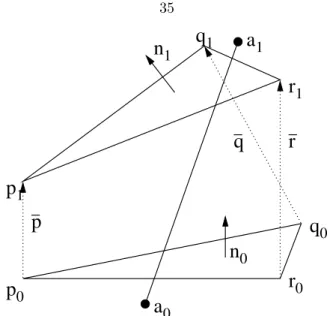
4.2 Identification of Crossover Points . . . 33
4.3 Event horizons from numerical simulations of binary black hole mergers . . . 36
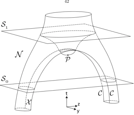
4.4 Topological structure of the Event Horizon for inspiraling and merging black holes . 38 4.5 Topological Structure of Simulated Event Horizons . . . 43
4.5.1 Equal-mass non-spinning merger . . . 44
4.5.2 2:1 mass ratio with ‘randomly’ oriented spins . . . 46
4.5.2.1 Pre-merger: t= 124.200M∗ . . . 47
4.5.2.2 Merger: t= 124.355M∗ . . . 49
4.5.2.3 Post-merger: t= 124.400M∗ . . . 49
4.5.3 Discussion on the numerical analysis of topological features . . . 53
4.6 Conclusion . . . 53
II Work with [that] matter[s] 58
5 Behavior of Pseudospectral Coefficients in the Presence of a Non-smoothness 59 5.1 Motivation . . . 595.2 Preliminaries and theoretical background . . . 60
5.2.1 Expected convergence of the metric at the stellar surface . . . 60
5.2.2 The ‘pseudo’ in pseudospectral methods . . . 61
5.2.3 Measures of the truncation error . . . 62
5.3 Methods . . . 62
5.4 Results . . . 63
5.5 Discussion and concluding remarks . . . 65
6 Simulations of neutron star-neutron star inspirals with SpEC 70 6.1 Introduction . . . 70
6.1.1 NSNS coalescence and gravitational waves . . . 70
6.1.2 Short gamma-ray bursts and other electromagnetic counterparts . . . 73
6.1.3 SpEC . . . 73
6.2 Methods and initial data . . . 74
6.2.1 Code details . . . 74
6.2.2 Initial data . . . 76
6.3 Results . . . 77
6.4 Discussion and conclusions . . . 79
7 Black hole formation from isolated neutron stars in SpEC 86 7.1 Literature review and introduction . . . 86
7.2 Methods and numerical setup . . . 87
7.2.1 Hydrodynamics grid . . . 87
7.2.2 Spectral grid and methods . . . 88
7.2.3 Time evolution and grid-to-grid communication . . . 88
7.2.4 Equation of state . . . 89
7.2.5 Hydrodynamic evolution equations . . . 89
7.2.6 Generalized harmonic equations . . . 91
7.2.7 Excision of nascent black hole . . . 91
7.3 Gauge equations, conditions, and methods . . . 92
7.3.1 Harmonic and generalized harmonic gauge . . . 92
7.3.2 Damped harmonic gauge for numerical evolutions . . . 93
7.3.3 Imposing damped harmonic gauge inSpEC simulations . . . 94
7.4 Initial Models and physical setup . . . 95
7.4.1 Methods . . . 95
7.4.2 Models . . . 96
7.4.3 Code parameters . . . 96
7.5 Results and discussion . . . 96
7.A Plots documenting the robustness of the simulations . . . 99
7.A.1 Convergence of simulations . . . 99
7.A.2 Gravitational waves from collapse . . . 99
7.B Definition of the 3-Velocity . . . 99
7.C Resolving the constraint equations . . . 102
8 The Influence of Thermal Pressure on Hypermassive Neutron Star Merger Rem- nants 107 8.1 Introduction . . . 108
8.2 Methods and Equations of State . . . 110
8.2.1 Equations of State . . . 110
8.2.2 Temperature and Composition Parametrizations . . . 115
8.2.3 Spherically Symmetric Equilibrium Models . . . 117
8.2.4 Axisymmetric Equilibrium Models . . . 117
8.3 Results: Spherically Symmetric Models . . . 119
8.4 Results: Axisymmetric Models in Rotational Equilibrium . . . 123
8.4.1 Uniformly Rotating Configurations . . . 123
8.4.2 Differentially Rotating Configurations . . . 125
8.5 Discussion and comparison with 3D NSNS simulations . . . 130
8.5.1 The Stability of HMNS Equilibrium Sequences . . . 130
8.5.2 The Secular Evolution of HMNS from Mergers . . . 132
8.5.3 Comparison with NSNS Merger Simulations . . . 134
8.6 Summary and Conclusions . . . 138
8.A Temperature Parametrizations . . . 141
8.B Solving for the Electron Fraction . . . 143
9 Supplements to The Influence of Thermal Pressure on Hypermassive Neutron Star Merger Remnants 150 9.1 Expanded discussion on the stability of HMNS equilibrium sequences . . . 150
9.1.1 Review on established applications of the turning-point method to neutron star stability . . . 150
9.1.2 Applying the turning-point method in more general cases . . . 153
9.1.3 Approximate turning points for alternate tuples of conserved quantities . . . 155
9.2 Properties of quasitoroidal models . . . 156
9.2.1 Criterion which implies a model must be quasitoroidal . . . 156
9.2.2 The fluid element atρb,maxis freely falling. . . 158
9.2.3 Maximum of the centrifugal support with differential rotation . . . 158
9.3 Changes in energy and density of a configuration . . . 159
9.4 Relation of average density to mass-shed centrifugal support . . . 160
9.5 Newtonian estimate of angular momentum at coalescence . . . 161
Chapter 1
Overview and historical summary
1.1 Introduction
The content of this thesis contains chapters of two different natures, both with the goal of sum- marizing the research I have accomplished during my time as a graduate student in the TAPIR (Theoretical AstroPhysics Including Relativity) group. One kind consists of works published or recently submitted for publication to which I have made a significant contribution: Chapters 2, 3, 4, and 8. These works are reproduced in their entirety, and my specific role in these works will be detailed here in Chapter 1. The other style of chapter contains work which is unpublished or unfinished work, involving the SpEC-hydro numerical relativity code (Chapters 5, 6 and 7). The primary goal of these chapters is to not only showcase the scientific results of this work, but also to document it so that SpEC-hydro researchers have a record of the numerical experiments I have conducted. Finally, Chapter 9 contains supplementary materials to the paper reproduced in Chapter 8.
The style of this overview chapter will be somewhat in in the form of a historical overview, as this will assist in detailing the specific contributions I have made to each work. It will also give me the chance to mention some non-scientific contributions which I feel have had a significant impact on the SXS collaboration.
1.2 Re: The Title or A Literary Aside
Though unconventional, the title of this thesis is appropriate on several levels. Tori is the plural of torus which is the mathematical term for a ‘donut’ shape; formally it defines a topology which is homeomorphic to the Cartesian product of two circles, S1 ×S1. In Chapter 4, we study the topological structure of event horizons in binary black hole mergers, and find no evidence for a toroidal (donut) shape. Chapter 8 examines equilibrium configurations of hypermassive neutron star remnants. Here, our investigations originally led us to believe that the enhancement seen
in the masses of these stellar configurations, due to differential rotation, was related to the stars beginning to take on a toroidal-like shape; these shapes, which look somewhat like that of a red-blood cell, are referred to as quasitoroidal. However, after further investigation, we found quasitoroidal morphologies to be astrophysically unrealistic configurations and not of great relevance to our study.
Hence, I’ve happened to conduct numerical studies of compact objects “Where Tori Fear to Tread.”
Additionally, the phrase is a reference to the famous line of the the poemAn Essay on Criticism by Alexander Pope: “For fools rush in where angels fear to tread.” The verse is a parable noting that the naive will often venture into situations that shrewd and more experienced will avoid. Directly applied to the studies I’ve conducted, this line could be twisted into the statement: “A fool may rush to the conclusion that toroidal shapes are significant to these topics; however a thorough investigation has revealed that tori are unimportant here.” However, I find the verse’s meaning to be personally significant as the parable represents perhaps the most important lesson I have learned during my graduate studies, that of the intrinsic value of experience. For me, this lesson takes many forms, one of which is the understanding that the hard work invested into tasks and projects which do not pan out is not wasted. Instead, such labor has intrinsic value in the experience it provides. The unstructured nature and long duration of graduate study is, essentially, for gaining experience in accomplishing tasks at the cutting edge of human knowledge. While many tasks and investigations in research may seem futile, pointless, or without motivation, perhaps such unstructured study is the only manner in which to prepare one for the task of uncovering new knowledge.
So I suppose it’s a good thing I went grad school, otherwise I’d be going around with the foolish impression that the outcome of compact object coalescence is some sort of toroidal structure...
1.3 Summary
1.3.1 Early work
My initial work in the TAPIR group consisted of research led by Kip Thorne and Yanbei Chen in developing methods of visualizing and understanding the spacetimes observed in numerical simula- tions of binary black hole mergers. The first approach to this involved using gauge dependent local measures of gravitational field energy and momentum, along with their respective integral conser- vation laws in an attempt to understand the dynamics of merging binary black holes. Chapter 2, originally published as [2] is a particular formulation of the post-Newtonian approximation in a form designed to resemble Maxwell’s equations in form and function. It was conceived and first organized by Kip Throne; David Nichols and I repeated and refined Kip’s calculations, and I presented the work at the April 2009 meeting of the American Physical Society.
I was also an author on the paper Momentum flow in black-hole binaries. II. Numerical simu- lations of equal-mass, head-on mergers with antiparallel spins [3], which is not reproduced in this
thesis. For this work, I was trained by Michael Cohen on the use of the event horizon finder which he wrote for the SpEC code. For the work, I calculated the event horizon for the SpEC head-on, anti-aligned spinning binary black hole merger simulated by Geoffrey Lovelace, as well as assisted in calculating the surface integral of field momentum over the event horizon surface. This calculation is illustrated in Figs. 13 and 14 of the work. Additionally, since the workflow for the event horizon finder code (from initial data generation through post-processing) was very much experimental at the time, I formalized and automated the process via scripts.
Another approach developed by our collaboration is that of representing the general relativistic gravitational field in terms of vortex and tendex lines. Chapter 3 reproduces our collaboration’s submission to Physical Review Letters [5]. Here I distinctly remember my contribution as checking the signs in the physical interpretations of the tidal and frame-drag fields (paragraph 2 of Sec. 3.1)!
I also contributed to the fine-tuning of Fig. 3.21, and the calculation of the event horizon surface in Fig. 3.1. The website companion pages; I did those too. Sincerely though, it was a pleasure and an honor to be a part of an analytical and numerical collaboration so talented that I could just barely keep up with their insights. Additionally, I was an author on the first in a series of follow up papers, which I have also chosen not to reproduce in this thesis [4].
1.3.2 Intermediate work: EH No Tori
Chapter 4 is a reproduction of the work published in Physical Review D entitled On Toroidal Horizons in Binary Black Hole Inspirals [1]. The work consisted of previously unpublished material in the thesis of Michael Cohen. The event-horizon finding code, algorithm for identification of crossover points, investigation of the equal-mass BBH merger and analysis of the generic topological structure of binary black hole mergers was done by Mike. Upon this solid foundation, my task was to examine the ‘generic’ BBH merger and verify that the conclusions drawn by Mike were robust. I accomplished this by calculating event horizon of the ‘generic’ merger for different spatial, temporal and simulation data resolutions. In addition, I thought carefully about what it would mean to resolve a topological feature of a numerical simulation. I subsequently developed a precise criterion for how one could, in principle, determine whether or not a numerically located event horizon shows evidence for the presence of a toroidal topology. Mark Scheel carefully examined our results and, as always, powered us through when code bugs became too challenging. To this date (almost two years later!), no one has found evidence for a toroidal event horizon in the slicing of their fully relativistic BBH merger simulations.
1particularly exciting was that this figure appeared on the cover of Physical Review Letters
1.3.3 SpEC-hydro work
In the spring of 2009, just before Christian Ott became an Assistant Professor at Caltech (at the time, he was a post-doc in the TAPIR group), he inquired if any student was interested in investigating neutron star-neutron star coalescence with the SpEC code. As a young grad student, I thought that this would be a good opportunity to use my experience with SpEC (at the time calculating event horizons) to work on research that had a wider range of astrophysical applications2. Later the following summer I shipped off to Cornell for a week to learn the methods of the budding SpEC-hydro code being written by Matt Duez and Francois Foucart. Conveniently enough, Curran Muhlberger had just written code to calculate NSNS initial data, and before October 2009, I was using SpEC-hydro to evolve some orbiting neutron stars. How, you might ask, did I end up in June of 2013 with no SpEC-hydro NSNS publication? Of course, there were distractions with the previously mentioned projects, and, uh... ‘general grad-studentyness’. However, I’d like to think that those were not the major reasons for the difficulty in progress with NSNSs inSpEC-hydro. Here I will explain my thoughts on the issue.
(I) The coupling of shock-capturing high-resolution finite-differencing methods and pseudospec- tral methods proved to be more delicate than was anticipated (cf. Ch. 5 for one example): it took nearly a year after first starting the simulations to achieve inspirals which were convergent in resolution. One problem identified here was that the PPM reconstruction scheme seemed to pro- duce gridpoint-to-gridpoint variations in the density. Once we switched to the smoother WENO reconstruction scheme, we started to make progress on the convergence issue.
(II) The development of the SpEC-hydro code rapidly diverged from many major practices in the vacuum SpEC code during its initial phases. To be frank, its development ended up somewhat rushed and without consideration for multiple users. That is, it was particularly specialized to BHNS coalescences. This issue seemed to stem from the fact that theSpEC code itself is a complex piece of software with a high learning curve. I never completely ‘dove in’ to theSpEC-hydro code, deconstructing it and voraciously determining its every nuance and feature. In retrospect, this is what I now feel would have been necessary to have generated more results. In an attempt to mitigate future student’s reluctance to ‘dive into’ theSpEC code, reduce bugs and propagate best practices, I took the initiative to lead the 2011 Summer SpEC coding class. The 9 week informal video conferenced course was a success: taught by Professors and Senior Researchers, approximately 20 students across more than four universities participated with a completion rate for the optional assignments of > 50%. Though this course could only scratch the surface of the SpEC code, the course materials are currently the standard for introducing new researchers to writing software for SpEC.
2get back to my roots, so to speak: in undergrad at Northwestern I conducted my undergraduate research in the theoretical astrophysics group under the guidance of Vicky Kalogera
(III) Communication and propagation of best practices across collaborating research groups proved difficult. For more than a year after starting the project, I was the only SpEC-hydro col- laborator who was not at Cornell (and for slightly more than two years I was the only SpEC-hydro collaborator at Caltech). Additionally, those who were readily available to advise me, were primar- ily focused on the vacuumSpEC code. This meant that I was primarily assisted by those who used the same codebase, but a very different branch of the code. One step I took in order to address the communication issue was to introduce the use of issue-tracking software to the collaboration.
Though the use of bug-tracking software was probably an inevitability for the collaboration, my initiative in its initial setup certainly hastened its arrival. The trac software I installed now has over 540 opened tickets, 420 closed tickets, and continues to be in active use by the collaboration.
(IV) Technical developments necessary for the robust simulation of NSNS coalescence needed to be accomplished. While the necessity of new technology is necessary for any experimental science, it was perhaps under-appreciated that new technical developments which were unique to the NSNS coalescence problem (i.e. not shared by the BHNS evolutions) had yet to be innovated. These included the ‘dual box’ regridder method, pushed by B´ela Szil´agyi and written by Francois Foucart.
This was necessary in order to accomplish the long inspiral which is the subject of Chapter 6.
Although, this subsequently required infrastructure (developed by Roland Haas) to merge the two grids into a single grid and continue evolution to black hole formation. Speaking of which, the formation of a new black hole is a good example of a phenomenon which may be present during the coalescence of two neutron stars, but is not present BHNS binaries. The technical feat of forming a new black hole inSpEC-hydro is the subject of Chapter 7.
1.3.4 On thermal effects in hypermassive neutron stars
In September of 2012, Christian Ott was inspired to investigate the subject of thermal pressure support in hypermassive neutron stars (HMNSs) via examining the maximum masses of neutron star equilibrium models for ‘hot’ temperatures (∼ 10s of MeV for neutron stars) using realistic tabulated equations of state. Originally intended to be a one week investigation, I was put to the task of calculating rotating equilibrium models of HMNS using the code of Cook, Shapiro and Teukolsky. Nine months later, the study has lead to perhaps the most interesting result included in this thesis. This study is the subject of the paper reproduced in Chapter 8, which is intended for submission to The Astrophysical Journal on the same date as the submission proofs of this thesis.
One of the first aspects I noticed of the properties of equilibrium models with significant differen- tial rotation was the correlation between very massive models withρb,maxaround nuclear saturation density (2.7×10¹⁴g/cm3) and aquasitoroidal morphology of the model. While, investigations into this correlation never matured into causation, I was still able to derive a few nice analytical results regarding the properties of quasitoroidal equilibrium models (cf. Sec. 9.2). The fundamental puzzle
we were exploring was that results in the literature of 3D NSNS simulations indicated that thermal support was important in stabilizing HMNSs from gravitational collapse. However the properties of the 1D and 2D equilibrium sequences we were calculating implied that thermal effects were es- sentiallyirrelevant to the maximum mass supported by rotation and the nuclear equation of state.
I was led to the resolution of this discrepancy through my efforts attempting to understand how one might reason about the stability of the equilibrium models we had constructed. This led me to construct sequences of constant baryonic mass models and examine a primitive version of Fig. 8.11.
Figure 8.11 shows that, for varied temperatures and magnitudes of differential rotation, all constant baryonic mass equilibrium sequences reach a minimum in their energy (gravitational mass) within a small window of maximum densities. After much blank staring at the figure, I came to the re- alization which was to become the major result of the work: a picture of the secular evolution of HMNSs in which this density regime should mark the transition from a stable HMNS to one which is unstable to gravitational collapse. With this new framework, we were able develop a coherent picture which reconciled the results found in the literature with those of our equilibrium models;
this work is discussed in Chapter 8.
Bibliography
[1] M. I. Cohen, J. D. Kaplan, and M. A. Scheel. Toroidal horizons in binary black hole inspirals.
Phys. Rev. D, 85(2):024031, January 2012.
[2] J. D. Kaplan, D. A. Nichols, and K. S. Thorne. Post-Newtonian approximation in Maxwell-like form. Phys. Rev. D, 80(12):124014, December 2009.
[3] G. Lovelace, Y. Chen, M. Cohen, J. D. Kaplan, D. Keppel, K. D. Matthews, D. A. Nichols, M. A.
Scheel, and U. Sperhake. Momentum flow in black-hole binaries. II. Numerical simulations of equal-mass, head-on mergers with antiparallel spins. Phys. Rev. D, 82(6):064031, September 2010.
[4] D. A. Nichols, R. Owen, F. Zhang, A. Zimmerman, J. Brink, Y. Chen, J. D. Kaplan, G. Lovelace, K. D. Matthews, M. A. Scheel, and K. S. Thorne. Visualizing spacetime curvature via frame- drag vortexes and tidal tendexes: General theory and weak-gravity applications. Phys. Rev. D, 84(12):124014, December 2011.
[5] R. Owen, J. Brink, Y. Chen, J. D. Kaplan, G. Lovelace, K. D. Matthews, D. A. Nichols, M. A.
Scheel, F. Zhang, A. Zimmerman, and K. S. Thorne. Frame-Dragging Vortexes and Tidal Ten- dexes Attached to Colliding Black Holes: Visualizing the Curvature of Spacetime. Physical Review Letters, 106(15):151101, April 2011.
Part I
Work in (a) vacuum
Chapter 2
Post-Newtonian Approximation in Maxwell-Like Form
The equations of thelinearizedfirst post-Newtonian approximation to general relativity are often written in “gravitoelectromagnetic” Maxwell-like form, since that facilitates physical intuition. Damour, Soffel and Xu (DSX) (as a side issue in their complex but el- egant papers on relativistic celestial mechanics) have expressed the first post-Newtonian approximation, including all nonlinearities, in Maxwell-like form. This paper summa- rizes that DSX Maxwell-like formalism (which is not easily extracted from their ce- lestial mechanics papers), and then extends it to include the post-Newtonian (Landau- Lifshitz-based) gravitational momentum density, momentum flux (i.e. gravitational stress tensor) and law of momentum conservation in Maxwell-like form. The authors and their colleagues have found these Maxwell-like momentum tools useful for developing physical intuition into numerical-relativity simulations of compact binaries with spin.
Originally published as Jeffrey D. Kaplan, David A. Nichols, and Kip S. Thorne. Post- Newtonian approximation in Maxwell-like form, Phys. Rev. D 80, 124014
2.1 Introduction
In 1961, Robert L. Forward [1] (building on earlier work of Einstein [2, 3] and especially Thirring [4, 5]) wrote the linearized, slow-motion approximation to general relativity in a form that closely resembles Maxwell’s equations; and he displayed this formulation’s great intuitive and computational power. In the half century since then, this Maxwell-like formulation and variants of it have been widely explored and used; see, e.g., [6–13] and references therein.
In 1965–69 S. Chandrasekhar [14, 15] formulated the first post-Newtonian (weak-gravity, slow- motion) approximation to general relativity in a manner that has been widely used for astrophysical
calculations during the subsequent 40 years. When linearized, this first post-Newtonian (1PN) approximation can be (and often is) recast in Maxwell-like form.
In 1991, T. Damour, M. Soffel and C. Xu (DSX; [16]) extended this Maxwell-like 1PN formalism to include all 1PN nonlinearities (see also Sec. 13 of Jantzen, Carini and Bini [17]). DSX did so as a tool in developing a general formalism for the celestial mechanics of bodies that have arbitrary internal structures and correspondingly have external gravitational fields characterized by two infi- nite sets of multipole moments. (For a generalization to scalar-tensor theories, see [18].) In 2004, Racine and Flanagan [19] generalized DSX to a system of compact bodies (e.g. black holes) that have arbitrarily strong internal gravity.
During the past 18 months, we and our colleagues have been exploring the flow of gravitational field momentum in numerical-relativity simulations of compact, spinning binaries [20, 21]. In their inspiral phase, these binaries’ motions and precessions can be described by the 1PN approximation,1 and we have gained much insight into their dynamics by using the 1PN DSX Maxwell-like formalism, extendedto include Maxwell-like momentum density, momentum flux, and momentum conservation.2 In this paper, we present that extension of DSX,3 though with two specializations: (i) we fix our coordinates (gauge) to be fully harmonic instead of maintaining the partial gauge invariance of DSX, and (ii) we discard all multipole moments of the binaries’ bodies except their masses and their spin angular momenta, because for black holes and neutron stars, the influences of all other moments are numerically much smaller than 1.5PN order.
The DSX celestial-mechanics papers [16, 22–24] are so long and complex that it is not easy to extract from them the bare essentials of the DSX Maxwell-like 1PN formalism. For the benefit of researchers who want those bare essentials and want to see how they are related to more conventional approaches to 1PN theory, we summarize them before presenting our momentum extension, and we do so for a general stress-energy tensor, for a perfect fluid, and for a system of compact bodies described by their masses and spins.
This paper is organized as follows: In Sec. 2.2 we summarize the basic DSX equations for 1PN theory in Maxwell-like form. In Sec. 2.3 we specialize the DSX formalism to a perfect fluid and make contact with the conventional 1PN notation. In Sec. 2.4 we extend DSX by deriving the (Landau- Lifshitz-based) density and flux of gravitational momentum in terms of the DSX gravitoelectric and gravitomagnetic fields and by writing down the law of momentum conservation in terms of them.
1For black-hole and neutron-star binaries, the influences of spin that interest us are formally 1PN, but because of the bodies’ compactness (size of order Schwarzschild radius), they are numerically 1.5PN.
2A referee has pointed out to us that some papers in the rich literature on the Maxwell-like formulation of linearized 1PN theory, e.g. [10], argue that the Maxwell analogy is physically useful only for stationary phenomena. Our spinning- binary application [20] of the momentum-generalized DSX formalism is a counterexample.
3When we carried out our analysis and wrote it up in the original version of this paper, we were unaware of the Maxwell-like formalism in DSX [16]; see our preprint athttp://xxx.lanl.gov/abs/0808.2510v1When we learned of DSX from Luc Blanchet, we used it to improve our Maxwell-like treatment of gravitational momentum (by replacing our definition for the gravitoelectric field by that of DSX) and we rewrote this paper to highlight the connection to DSX.
(It is this that we have found so useful for gaining intuition into numerical-relativity simulations of inspiraling, spinning binaries [20, 21].) In Sec. 2.5 we briefly discuss energy conservation. In Sec. 2.6, relying on Racine and Flanagan [19], we specialize to the vacuum in the near zone of a system made from compact bodies with arbitrarily strong internal gravity. Finally, in Sec. 2.7 we summarize the DSX formalism and our extension of it both for a self-gravitating fluid and for a system of compact bodies.
Throughout this paper, we set G=c = 1, Greek letters run from 0 to 3 (spacetime) and Latin from 1 to 3 (space), and we use the notation of field theory in flat space in a 3+1 split, so spatial indices are placed up or down equivalently and repeated spatial indices are summed whether up or down or mixed. We use bold-face italic characters to represent spatial vectors, i.e.wis the bold-face version ofwj.
2.2 The DSX Maxwell-Like Formulation of 1PN Theory
Damour, Soffel and Xu (DSX [16]) express the 1PN metric in terms of two gravitational potentials, a scalarwand a vectorwj:
g00 = −e−2w=−1 + 2w−2w2+O(UN3),
g0i = −4wi+O(UN5/2), (2.1)
gij = δije2w=δij(1 + 2w) +O(UN2)
[DSX Eqs. (3.3)]. The Newtonian limit ofwisUN = (Newtonian gravitational potential), andwi is of orderUN3/2:
w=UN +O(UN2), wi =O(UN3/2). (2.2) The harmonic gauge condition implies that
w,t+wj,j = 0 (2.3)
[DSX Eq. (3.17a)]; here and throughout commas denote partial derivatives. Using this gauge con- dition (which DSX do not impose), the 1PN Einstein field equations take the following remarkably simple form:
∇2w−w¨ = −4π(T00+Tjj) +O(UN3/L2), (2.4a)
∇2wi = −4πT0i+O(UN5/2/L2) (2.4b)
[DSX Eqs. (3.11)]. HereTαβis the stress-energy tensor of the source (which we specialize below to
a perfect fluid),∇2is the flat-space Laplacian (i.e.∇2w=w,jj), repeated indices are summed, dots denote time derivatives (i.e. ¨w=w,tt), andLis the lengthscale on whichwvaries.
Following DSX, we introduce the 1PNgravitoelectric fieldg(denotedeorEby DSX , depending on the context) andgravitomagnetic field H (denotedborB by DSX):
g = ∇w+ 4 ˙w+O(UN3/L), (2.5a)
H = −4∇×w+O(UN5/2/L). (2.5b)
[DSX Eqs. (3.21)].
The Einstein equations (2.4) and these definitions imply the following 1PN Maxwell-like equations forg andH:
∇·g = −4π(T00+Tjj)−3 ¨w+O(gUN2/L), (2.6a)
∇×g = −H˙ +O(gUN2/L), (2.6b)
∇·H = 0 +O(HUN/L), (2.6c)
∇×H = −16πT0iei+ 4 ˙g+O(HUN/L) (2.6d)
[DSX Eqs. (3.22)]. Hereeiis the unit vector in the idirection.
In terms ofgandH, the geodesic equation for a particle with ordinary velocityv=dx/dttakes the following form [Eq. (7.17) of DSX, though in a less transparently “Lorentz-force”-like form there]:
d dt
1 + 3UN+12v2 v
= 1−UN+32v2
g+v×H
+O(gUN2). (2.7)
Note that the spatial part of the particle’s 4-momentum is mu = m(1 +UN + 12v2)v at 1PN order. This accounts for the coefficient 1 +UN + 12v2 on the left-hand side of Eq. (2.7). The remaining factor 2UN is related to the difference between physical lengths and times, and proper lengths and times. In the linearized, very-low-velocity approximation, this geodesic equation takes the “Lorentz-force” formdv/dt=g+v×H, first deduced (so far as we know) in 1918 by Thirring [4], motivated by Einstein’s 1913 [2] insights about similarities between electromagnetic theory and his not-yet-perfected general relativity theory.
The 1PN deviations of the geodesic equation (2.7) from the usual Lorentz-force form might make one wonder about the efficacy of the DSX definition ofg. That efficacy will show up most strongly when we explore the gravitational momentum density in Sec. 2.4 below.
2.3 Specialization to a Perfect Fluid
We now depart from DSX by specializing our source to a perfect fluid and making contact with a set of 1PN gravitational potentials that are widely used. We pay special attention to connections with a paper by Pati and Will [27] because that paper will be our foundation, in Sec. 2.4, for computing the density and flux of gravitational field momentum.
We describe our perfect fluid in the following standard notation: ρo = (density of rest mass), Π =(internal energy per unit rest mass, i.e. specific internal energy),P = (pressure), all as measured in the fluid’s local rest frame;vj ≡dxj/dt= (fluid’s coordinate velocity).
Following Blanchet and Damour [28], and subsequently Pati and Will (Eqs. (4.13), (4.3) of [27]), we introduce a post-Newtonian variantU of the Newtonian potential, which is sourced byT00+Tjj:
∇2U =−4π(T00+Tjj). Accurate to 1PN order, the source is [see Eq. (2.18d)]
T00+Tjj =ρo(1 + Π + 2v2+ 2UN + 3P/ρo), (2.8) whereUN is the Newtonian limit ofU
UN(x, t) =
Z ρo(x0, t)
|x−x0|d3x0 . (2.9a)
Correspondingly,U can be written as
U =
Z ρo(1 + Π + 2v2+ 2UN + 3P/ρo)
|x−x0| d3x0. (2.9b)
Here and below the fluid variables and gravitational potentials in the integrand are functions of (x0, t) as in Eq. (2.9a). In Eq. (2.9a) forUN, ρo can be replaced by any quantity that agrees with ρo in the Newtonian limit, e.g. by the post-Newtonian “conserved mass density”ρ∗ of Eq. (2.13b) below. We also introduce Chandrasekhar’s Post-Newtonian scalar gravitational potential χ (Eq.
(44) of [14]), which is sourced by 2UN, ∇2χ=−2UN or equivalently
χ=− Z
ρo|x−x0|d3x0. (2.10)
Pati and Will use the notation−X forχ (Eqs. (4.14), (4.12a) and (4.3) of [27]).
It is straightforward to show that the 1PN solution to the wave equation (2.4a) for the DSX scalar potentialwis
w=U−1
2χ¨; (2.11)
and the 1PN solution to the Laplace equation (2.4b) for the DSX vector potentialwj is
wj=
Z ρovj
|x−x0|d3x0 . (2.12)
The fluid’s evolution is governed by rest-mass conservation, momentum conservation, and energy conservation.
The 1PN version of rest-mass conservation takes the following form:
ρ∗,t+∇·(ρ∗v) = 0, (2.13a) where
ρ∗=ρou0√
−g=ρo(1 +12v2+ 3U) (2.13b) (Eqs. (117) and (118) of Chandrasekhar [14]). Hereu0is the time component of the fluid’s 4-velocity andg is the determinant of the covariant components of the metric.
We shall discuss momentum conservation and energy conservation in the next two sections.
We note in passing that Chandrasekhar and many other researchers write their 1PN spacetime metric in a different gauge from our harmonic one. The two gauges are related by a change of time coordinate
tC=tH−12χ ,˙ (2.14a)
and correspondingly the metric components in the two gauges are related by
gC00=g00H + ¨χ , gC0j=gH0j+12χ˙,j . (2.14b) Here C refers to the Chandrasekhar gauge and H to our harmonic gauge. DSX write their equations in forms that are invariant under the gauge change (2.14).
2.4 Momentum Density, Flux, and Conservation
We now turn to our extension of the DSX formalism to include a Maxwell-like formulation of gravita- tional momentum density, momentum flux, and momentum conservation. Following Chandrasekhar [15], Pati and Will [27] and others, we adopt the Landau-Lifshitz pseudotensor as our tool for formulating these concepts.
From Pati and Will’s 2PN harmonic-gauge Eqs. (2.6), (4.4b) and (4.4c) for the pseudotensor, one can deduce the following 1PN expressions for the the gravitational momentum density and
momentum flux (stress) in terms of the DSX gravitoelectric and gravitomagnetic fieldsg andH:
(−g)t0jLLej = −4π1g×H+4π3U˙Ng,
(2.15a) (−g)tijLL = 4π1(gigj−12δijgkgk)
+16π1 (HiHj−12δijHkHk)−8π3U˙N2δij.
(2.15b)
Each equation is accurate up to corrections of order UN times the smallest term on the right side (2PN corrections).
For comparison, in flat spacetime the electromagnetic momentum density is 4π1E×B and the momentum flux is4π1(EiEj−12δijEkEk)+4π1 (BiBj−12δijBkBk). Aside from a sign in Eq. (2.15a) and the two terms involvingU˙N, the gravitational momentum flux and density (2.15) are identical to the electromagnetic ones withE→gandB→H. Therefore, by analogy with the electromagnetic case, there aregravitational tensions|g|2/8πand|H|2/8πparallel to gravitoelectric and gravitomagnetic field lines, and gravitational pressures of this same magnitude orthogonal to the field lines. This makes the gravitoelectric and gravitomagnetic fieldsgandHpowerful tools for building up physical intuition about the distribution and flow of gravitational momentum. We use them for that in our studies of compact binaries [20], relying heavily on Eqs. (2.15).
Here are some hints for deducing Eqs. (2.15) from Pati and Will [27] (henceforth PW): (i) Show that the last two terms in (2.6) of PW are of 2PN order for{α, β} ={0j} or {ij} and so can be ignored, whence 16π(−g)tαβLL= Λαβ. (ii) Show that our notation is related to that of PW byχ=−X, U the same,w=U−12χ¨=14(N+B)−18(N+B)2[for the last of these cf. PW (5.2), (5.4a,c)], and at Newtonian orderUN = 14N. (iii) In PW (4.4b,c) for Λαβ, keep only the Newtonian and 1PN terms:
the first curly bracket in (4.4b) and first and second curly brackets in (4.4c). Rearrange those terms so they involve onlyK, N+B and the Newtonian-order N, use the above translation of notation and use the definitions (2.5) ofgandH. Thereby, bring PW (4.4b,c) into the form (2.15).
In the Landau-Lifshitz formalism, the local law of 4-momentum conservation Tjµ;µ = 0 takes the form
[(−g)(Tjµ+tjµLL)],µ= 0 (2.16) (Eqs. (20.23a) and (20.19) of [29], or (100.8) of [30]). Here (as usual), commas denote partial derivatives, and semicolons denote covariant derivatives. This is the conservation law that we use in our studies of momentum flow in compact binaries [20].
When dealing with material bodies (e.g. in DSX) rather than with the vacuum outside compact bodies, an alternative Maxwell-like version of momentum conservation is useful. Specifically, using
expressions (2.15) and (−g) = 1 + 4UN [from Eq. (2.1) with w=UN at leading order], and using the field equations (2.6) forg andH, the conservation law (2.16) can be rewritten in the following simple Lorentz-force-like form (Eq. (4.3) of Damour, Soffel and Xu’s Paper II [22])
[(1 + 4UN)Ti0],t+ [(1 + 4UN)Tij],j (2.17)
= (T00+Tjj)gi+ijkT0jHk.
Here the Levi-Civita tensorijk produces a cross product of the momentum density with the grav- itomagnetic field. For comparison, in flat spacetime, the momentum conservation law for a charged medium interacting with electric and magnetic fields Ei and Bi has the form Ti0,t +Tij,j = ρeEi +ijkJjBk, where ρe is the charge density and Jj the charge flux (current density). The right-hand side of Eq. (2.17) (the gravitational force density) is identical to that in the electromag- netic case, with ρe→ (T00+Tjj), Jj →T0j, E →g, and B →H. Again, this makes g and H powerful foundations for gravitational intuition.
For a perfect fluid, the components of the 1PN stress-energy tensor, which appear in the mo- mentum conservation law (2.17), are (Eqs. (20) of Chandrasekhar [14])
T00 = ρo(1 + Π +v2+ 2UN), (2.18a)
Ti0 = ρo(1 + Π +v2+ 2UN +P/ρo)vj, (2.18b) Tij = ρo(1 + Π +v2+ 2UN+P/ρo)vivj
+P(1−2UN)δij, (2.18c)
T00+Tjj = ρ(1 + Π + 2v2+ 2UN + 3P/ρo). (2.18d)
2.5 Energy Conservation
For a perfect fluid, the exact (not just 1PN) law of energy conservation, when combined with mass conservation and momentum conservation, reduces to the first law of thermodynamics dΠ/dt =
−P d(1/ρo)/dt; so whenever one needs to invoke energy conservation, the first law is the simplest way to do so. For this reason, and because deriving the explicit form of 1PN energy conservation [(−g)(T0µ+t0µLL)],µ= 0 is a very complex and delicate task (cf. Sec. VI of [31]), we shall not write it down here.
However, wedowrite down the Newtonian law of energy conservation in harmonic gauge, since we will occasionally need it in our future papers. Chandrasekhar calculated (−g)(T0µ+t0µLL) in [15]; his Eqs. (48) and (57) are the time-time and time-space components, respectively. When one
writes the expressions in terms of the “conserved rest-mass density” ρ∗ [Eq. (2.13b)] and in our Maxwell-like form, Newtonian conservation of energy states that
ρ∗(1 + Π +1
2v2+ 3UN)− 7 8πg·g
,t
+∇·
ρ∗v(1 + Π +P ρ +1
2v2+ 3UN) + 3
4πU˙Ng− 1 4πg×H
= 0. (2.19)
While this equation is perfectly correct, it expresses Newtonian energy conservation in terms of the post-Newtonian gravitomagnetic fieldH. It is possible to rewrite theH-dependent term using the relationship, ∇ ·[−1/(4π)(g×H)] = ∇ ·[−4UNT0jej+ (1/π)UNg], which is accurate up to˙ corrections of orderg·H. This relationship can be found by applying Eq. (2.6b) once and (2.6d)˙ twice, in combination with elementary vector-calculus identities. The statement of Newtonian energy conservation then depends only upon the Newtonian potential and its gradient and time derivative:
ρ∗(1 + Π +1
2v2+ 3UN)− 7 8πg·g
,t
+∇·
ρ∗v(1 + Π +P ρ +1
2v2−UN) + 3
4πU˙Ng+ 1 πUNg˙
= 0. (2.20)
Notice that going from Eq. (2.19) to Eq. (2.20) involves adding a divergence-free piece to the energy flux, so it entails changing how the energy flux is localized — a change that strictly speaking takes the energy flux out of harmonic gauge.
If the coefficients of the gravitational terms in Eq. (2.20) look unfamiliar, it is because even at Newtonian order, the density and flux of gravitational energy are gauge-dependent. In some other gauge, they will be different; see Box 12.3 of [32].
2.6 Gravitational Potentials in the Vacuum of a System of Compact, Spinning Bodies
For a system of compact, spinning bodies (neutron stars or black holes), the gravitational potentials UN,U, wi andχ in the vacuum between the bodies take the following forms (in a slightly different
harmonic gauge than the one used in Sec. 2.3 for fluids):
UN = X
A
MA
rA
, (2.21a)
U = X
A
MA rA
1 +32vA2 − X
B6=A
MB rAB
+2X
A
ijkvAiSAjnkA
rA2 , (2.21b)
χ = −X
A
MArA, (2.21c)
w = U−1
2χ ,¨ (2.21d)
wi = X
A
MAviA rA
+1 2
X
A
ijkSAjnkA
rA2 , (2.21e)
Here the notation is that of Sec. IV of Thorne and Hartle [26]: the sum is over the compact bodies labeled by capital Latin letters A, B; MA, SAj and vAj are the mass, spin angular momentum and coordinate velocity of body A; rA is the coordinate distance from the field point to the center of mass of body A; rAB is the coordinate distance between the centers of mass of bodies A and B;
njA is the unit vector pointing from the center of mass of bodyA to the field point; andijk is the Levi-Civita tensor.
Equations (2.21) for the potentials can be deduced by comparing our 1PN spacetime metric coefficients [Eqs. (2.1), (2.11)] with those in Eqs. (2.4), (5.11) and (5.14) of Racine and Flanagan [19] or in Eqs. (4.4) of Thorne and Hartle [26].4
2.7 Conclusion
In our Maxwell-like formulation of the 1PN approximation to general relativity for fluid bodies, the evolution of the fluid and gravitational fields is governed by: (i) the law of momentum conservation (2.17), (2.18) (which can be thought of as evolving the fluid velocity vj); (ii) the law of mass conservation (2.13) (which can be thought of as evolving the mass densityρo); (iii) the equation of stateP(ρo) and first law of thermodynamicsdΠ =−P d(1/ρo) (which determineP and Π once ρo
is known); Eqs. (2.9), (2.12), (2.10) for the gravitational potentialsU,χ, and wj; and Eqs. (2.5) or (2.6) for the gravitoelectric and gravitomagnetic fieldsg,H.
4Racine and Flanagan specialize DSX to a system of compact bodies with a complete set of nonzero multipole moments. We neglect all moments except the bodies’ masses and spins (see fifth paragraph of Sec. 2.1). Our notation is related to that of Racine and Flanagan byUN=−Φ,w=U−1
2χ¨=−(Φ +ψ), wi=−1
4ζi. The Racine-Flanagan derivation of Eqs. (2.21) avoids considering the internal structures of the bodies and it therefore is directly valid for black holes. The Thorne-Hartle derivation relies on the pioneering analysis of Einstein, Infeld and Hoffman [33] which uses a fluid description of the bodies’ interiors. Thorne and Hartle extend Eqs. (2.21) to black holes by the equivalent of Damour’s “effacement” considerations, Sec. 6.4 of [25].
When specialized to a system of compact bodies, e.g. a binary made of black holes or neutron stars, the system is governed by: (i) 1PN equations of motion and precession for the binary (not given in this paper; see, e.g., Eqs. (4.10), (4.11) and (4.14) of [26]); (ii) momentum flow within the binary as described by the Landau-Lifshitz pseudotensor (2.15) and its conservation law (2.16), in which the gravitoelectric and gravitomagnetic fields are expressed as sums over the bodies via Eqs.
(2.21) and (2.5); and (iii) other tools developed by Landau and Lifshitz (Sec. 100 of [30]). We are finding this formalism powerful in gaining insight into compact binaries [20].
Acknowledgments
For helpful discussions we thank Yanbei Chen and Drew Keppel. We also thank Luc Blanchet for bringing references [28] and [16] to our attention, and anonymous referees for helpful critiques and suggestions. This research was supported in part by NSF grants PHY-0601459 and PHY-0653653 and by a Caltech Feynman Fellowship to JDK.
Bibliography
[1] R. L. Forward, Proc. IRE 49, 892 (1961).
[2] A. Einstein, Phys. Z. 14, 1261 (1913).
[3] A. Einstein, Four Lectures on the Theory of Relativity held at Princeton University in May 1921, English Translation by Edwin Plimpton Adams (London, Meutuen, 1922; Princeton Uni- versity Press, 1923); reproduced as Document 71 inThe Collected Papers of Albert Einstein,7 (Princeton University Press, 2002); see pp. 100–103.
[4] H. Thirring, Phys. Z.19, 204 (1918).
[5] H. Thirring, Phys. Z. 19, 33 (1918); and H. Thirring and J. Lense, Phys. Z. 19, 156 (1918);
English translations in B. Mashhoon, F.W. Hehl and D. S. Theiss, Gen. Rel. Grav. 16, 711 (1984).
[6] V. B. Braginsky, C. M. Caves and K. S. Thorne, Phys. Rev. D 15, 2047 (1977).
[7] R. M. Wald, General Relativity(University of Chicago Press, Chicago, 1984), Sec. 4.4a.
[8] B. Mashhoon, Phys. Lett. A 173, 347 (1993).
[9] B. Mashhoon, F. Gronwald and H. I. M. Lichtenegger, Lect. Notes Phys. 562, 83 (2001).
[10] S. J. Clark and R. W. Tucker, Class. Quant. Grav.17, 4125 (2000).
[11] B. Mashhoon, Class. Quant. Grav.25085014 (2008).
[12] E. Goulart and F. T. Falciano, J. Gen. Rel. Grav., submitted; arXiv:0807.2777 [13] L. F. O. Costa and C. A. R. Herdeiro Phys. Rev. D78, 024021 (2008).
[14] S. Chandrasekhar, Astrophys. J. 142, 1488 (1965); also available as Paper 6 in S. Chan- drasekhar,Selected Papers, Volume 5, Relativistic Astrophysics (University of Chicago Press, Chicago, 1990).
[15] S. Chandrasekhar, Astrophys. J.158, 45 (1969); also available as Paper 7 in S. Chandrasekhar, Selected Papers, Volume 5, Relativistic Astrophysics (University of Chicago Press, Chicago, 1990).
[16] T. Damour, M. Soffel, C. Xu, Phys. Rev. D43, 3273 (1991).
[17] R.T. Jantzen, P. Carini and D. Bini, Ass. Phys.215, 1 (1992).
[18] S. Kopeikin and I. Vlasov, Phys. Reports400, 209 (2004).
[19] E. Racine and E.E. Flanagan, Phys. Rev. D71, 044010 (2005).
[20] Y. Chen, D. G. Keppel, D. A. Nichols and K. S. Thorne, Phys. Rev. D, submitted (2009);
arXiv:0902.4077.
[21] G. Lovelace, Y. Chen, M. Cohen, J.D. Kaplan, D. Keppel, K.D. Matthews, D.A. Nichols, M.A.
Scheel, and U. Sperhake, Phys. Rev. D, submitted (2009); arXiv:0907.0869.
[22] T. Damour, M. Soffel, C. Xu, Phys. Rev. D45, 1017 (1992).
[23] T. Damour, M. Soffel, C. Xu, Phys. Rev. D47, 3124 (1993).
[24] T. Damour, M. Soffel, C. Xu, Phys. Rev. D49, 618 (1994).
[25] T. Damour, Chapter 6 inThree Hundred Years of Gravitation, eds. S.W. Hawking and W. Israel (Cambridge University Press, Cambridge, 1987).
[26] K. S. Thorne and J. B. Hartle, Phys. Rev. D31, 1815 (1985).
[27] M. E. Pati and C. M. Will, Phys. Rev. D62, 124015 (2000).
[28] L. Blanchet, T. Damour, Ann. Inst. Henri Poincar´e,50, 337 (1989).
[29] C. W. Misner, K. S. Thorne and J. A. Wheeler, Gravitation (W.H. Freeman, San Francisco, 1973).
[30] L. D. Landau and E.M. Lifshitz, Classical Theory of Fields(Addison Wesley, Redding Mass., 1962).
[31] S. Chandrasekhar and Y. Nutku, Astrophys. J. 158, 55 (1969); also available as Paper 8 in S. Chandrasekhar,Selected Papers, Volume5, Relativistic Astrophysics(University of Chicago Press, Chicago, 1990).
[32] R. D. Blandford and K. S. Thorne,Applications of Classical Physics(2009), available athttp:
//www.pma.caltech.edu/Courses/ph136/yr2008/.
[33] A. Einstein, L. Infeld and B. Hoffman, Ann. Math. 39, 65 (1938).
Chapter 3
Frame-Dragging Vortexes and Tidal Tendexes Attached to Colliding Black Holes:
Visualizing the Curvature of Spacetime
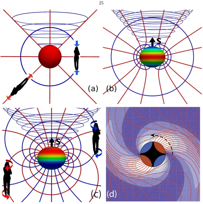
When one splits spacetime into space plus time, the spacetime curvature (Weyl tensor) gets split into an “electric” part Ejk that describes tidal gravity and a “magnetic” part Bjk that describes differential dragging of inertial frames. We introduce tools for visu- alizing Bjk (frame-drag vortex lines, their vorticity, and vortexes) andEjk (tidal tendex lines, their tendicity, and tendexes), and also visualizations of a black-hole horizon’s (scalar) vorticity and tendicity. We use these tools to elucidate the nonlinear dynamics of curved spacetime in merging black-hole binaries.
Originally published as Robert Owen, Jeandrew Brink, Yanbei Chen, Jeffrey D. Kaplan, Geoffrey Lovelace, Keith D. Matthews, David A. Nichols, Mark A. Scheel, Fan Zhang, Aaron Zimmerman, and Kip S. Thorne. Phys. Rev. Lett. 106, 151101 (2011)
3.1 Introduction
When one foliates spacetime with spacelike hypersurfaces, the Weyl curvature tensorCαβγδ(same as Riemann in vacuum) splits into “electric” and “magnetic” partsEjk=Cˆ0jˆ0k andBjk= 12jpqCpqkˆ0
(see e.g. [1] and references therein); bothEjk and Bjk are spatial, symmetric, and trace-free. Here the indices are in the reference frame of “orthogonal observers” who move orthogonal to the space slices; ˆ0 is their time component, jpq is their spatial Levi-Civita tensor, and throughout we use
units withc=G= 1.
Because two orthogonal observers separated by a tiny spatial vectorξexperience a relative tidal acceleration ∆aj =−Ejkξk, Ejk is called the tidal field. And because a gyroscope at the tip of ξ precesses due to frame dragging with an angular velocity ∆Ωj =Bjkξk relative to inertial frames at the tail ofξ, we callBjk theframe-drag field.
3.2 Vortexes and Tendexes in Black-Hole Horizons
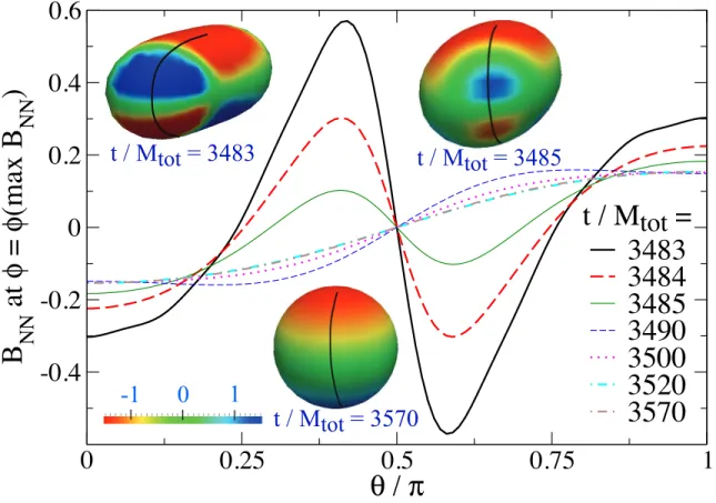
For a binary black hole, our space slices intersect the 3-dimensional (3D) event horizon in a 2D horizon with inward unit normalN; soBN N is the rate the frame-drag angular velocity around N increases as one moves inward through the horizon. Because of the connection between rotation and vorticity, we callBN N the horizon’sframe-drag vorticity, or simply itsvorticity.
Because BN N is boost-invariant alongN [2], the horizon’s vorticity is independent of how fast the orthogonal observers fall through the horizon, and is even unchanged if the observers hover immediately above the horizon (the FIDOs of the “black-hole membrane paradigm” [3]).
Figure 3.1 shows snapshots of the horizon for two identical black holes with transverse, oppositely directed spinsS, colliding head on. Before the collision, each horizon has a negative-vorticity region (red) centered onS, and a positive-vorticity region (blue) on the other side. We call these regions of concentrated vorticityhorizon vortexes. Our numerical simulation [4] shows the four vortexes being transferred to the merged horizon (Fig. 3.1b), then retaining their identities, but sloshing between positive and negative vorticity and gradually dying, as the hole settles into its final Schwarzschild state; see the movie in Ref. [5].
Because EN N measures the strength of the tidal-stretching acceleration felt by orthogonal ob- servers as they fall through (or hover above) the horizon, we call it the horizon’stendicity(a word coined by David Nichols from the Latin tendere, “to stretch”). On the two ends of the merged horizon in Fig. 3.1b there are regions of strongly enhanced tendicity, called tendexes; cf. Fig. 3.5
Figure 3.1: Vortexes (with positive vorticity blue, negative vorticity red) on the 2D event horizons of spinning, colliding black holes, just before and just after merger. (From the simulation reported in [4].)
below.
An orthogonal observer falling through the horizon carries an orthonormal tetrad consisting of her 4-velocity U, the horizon’s inward normal N, and transverse vectors e2 and e3. In the null tetradl= (U−N)/√
2 (tangent to horizon generators),n= (U+N)/√
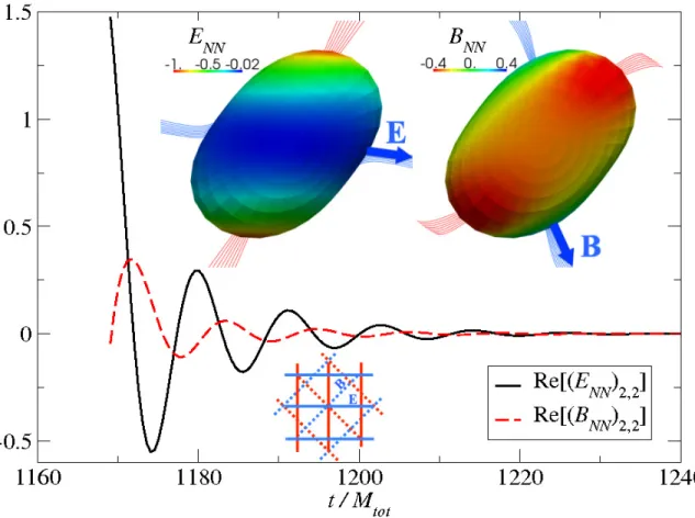
2,m= (e2+ie3)/√ 2, and m∗, the Newman-Penrose Weyl scalar Ψ2[6] is Ψ2= (EN N+iBN N)/2. Here we use sign conventions of [7], appropriate for our (- +++) signature.
Penrose and Rindler [8] define a complex scalar curvatureK=R/4+iX/4 of the 2D horizon, with Rits intrinsic (Ricci) scalar curvature (which characterizes the horizon’s shape) andX proportional to the 2D curl of its H´aj´ıˇcek field [9] (the space-time part of the 3D horizon’s extrinsic curvature).
Penrose and Rindler show thatK=−Ψ2+µρ−λσ, whereρ,σ,µ, andλare spin coefficients related to the expansion and shear of the null vectors l and n, respectively. In the limit of a shear- and expansion-free horizon (e.g. a quiescent black hole; Fig. 3.2a,b,c), µρ−λσ vanishes, so K =−Ψ2, whence R=−2EN N and X =−2BN N. As the dimensionless spin parameter a/M of a quiescent (Kerr) black hole is increased, the scalar curvature R= −2EN N at its poles decreases, becoming negative for a/M > √
3/2; see the blue spots on the poles in Fig. 3.2b compared to solid red for the nonrotating hole in Fig. 3.2a. In our binary-black-hole simulations, the contributions of the spin coefficients to K on the apparent horizons are small [L2-norm . 1%] so R ' −2EN N and X ' −2BN N, except for a time interval∼5Mtotnear merger. HereMtot is the binary’s total mass.
On the event horizon, the duration of spin-coefficient contributions >1% is somewhat longer, but we do not yet have a good measure of it.
Because X is the 2D curl of a 2D vector, its integral over the 2D horizon vanishes. Therefore, positive-vorticity regions must be balanced by negative-vorticity regions; it is impossible to have a horizon with just one vortex. By contrast, the Gauss-Bonnet theorem says the integral of R over the 2D horizon is 8π (assuming S2 topology), which implies the horizon tendicity EN N is predominantly negative (becauseEN N ' −R/2 andRis predominantly positive). Many black holes have negative horizon tendicity everywhere (an exception is Fig. 3.2b), so their horizon tendexes must be distinguished by deviations ofEN N from a horizon-averaged value.
3.3 3D vortex and tendex lines
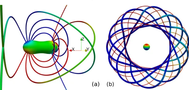
The frame-drag fieldBjk is symmetric and trace free and therefore is fully characterized by its three orthonormal eigenvectors e˜j and their eigenvalues B˜1˜1, B˜2˜2 and B˜3˜3. We call the integral curves alonge˜j vortex lines, and their eigenvalueB˜j˜j those lines’vorticity, and we call a concentration of vortex lines with large vorticity avortex. For the tidal fieldEjk the analogous quantities aretendex lines, tendicityand tendexes. For a nonrotating (Schwarzschild) black hole, we show a few tendex lines in Fig. 3.2a; and for a rapidly-spinning black hole (Kerr metric with a/M = 0.95) we show
tendex lines in Fig. 3.2b and vortex lines in Fig. 3.2c.
If a person’s body (with length `) is oriented along a positive-tendicity tendex line (blue in Fig.
3.2a), she feels a head-to-foot compressional acceleration ∆a =|tendicity|`; for negative tendicity (red) it is a stretch. If her body is oriented along a positive-vorticity vortex line (blue in Fig. 3.2c), her head sees a gyroscope at her feet precess clockwise with angular speed ∆Ω = |vorticity|`, and her feet see a gyroscope at her head also precess clockwise at the same rate. For negative vorticity (red) the precessions are counterclockwise.
For a nonrotating black hole, the stretching tendex lines are radial, and the squeezing ones lie on spheres (Fig. 3.2a). When the hole is spun up to a/M = 0.95 (Fig. 3.2b), its toroidal tendex lines acquire a spiral, and its poloidal tendex lines, when emerging from one polar region, return to the other polar region. For any spinning Kerr hole (e.g. Fig. 3.2c), the vortex lines from each polar region reach around the hole and return to the same region. The red vortex lines from the red north polar region constitute acounterclockwise vortex: the blue ones from the south polar region constitute aclockwise vortex.
As a dynamical example, consid