Identification of Neuronal Microcircuits

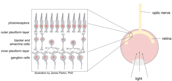
We also present the practicality of the technique in a case study of circuits in the mouse retina. Bipolar cell bodies reside in the inner nuclear layer and are the main excitatory interneuron of the retina (Figure 1.1).

Figure 1.1: Illustration of the structure of the retina.

Past applications of deep learning to visual neuroscience

Series stacking of LN units can not only successfully predict the output of ganglion cell layers, but also provides a mechanistic explanation for the type of feature selectivity often seen in retinal circuits.

System identification and structure recovery

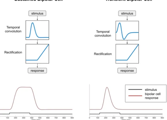
Based on the shape of the temporal filter, it is possible to produce a sustained or transient response (red lines) to a 250 ms light flash stimulus (black lines). The ganglion cell responds to the appearance of the spot, then adapts and becomes silent. In the case of a spreading stimulus, the ganglion cell fires again during this second phase of the stimulus.

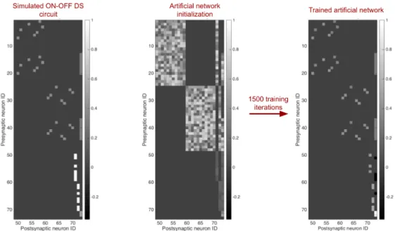
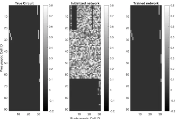
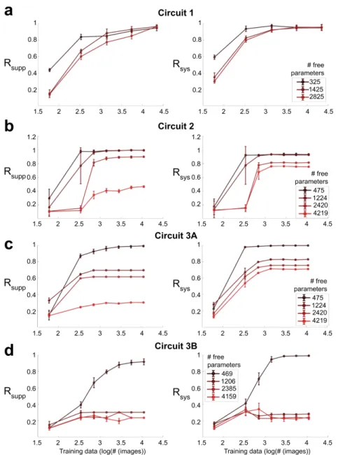
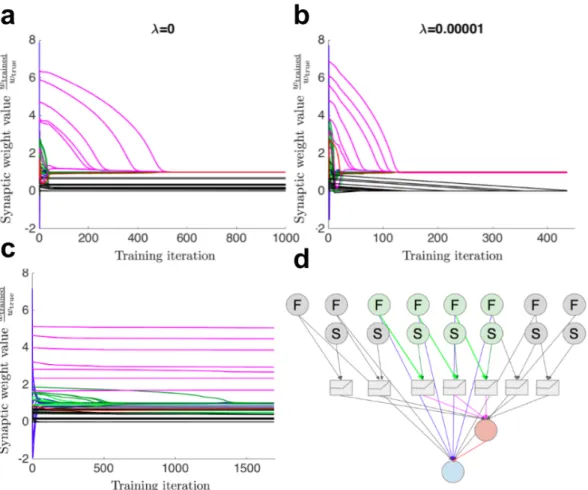
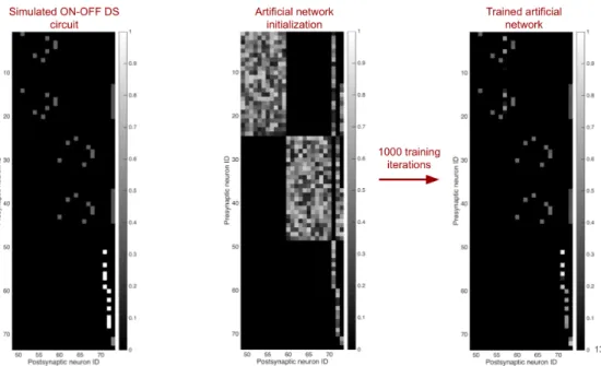
The basic connectivity motif of the true model was preserved in the trained model initialization (Fig. 4.9). Not surprisingly, system identification of all four circuits showed a strong dependence on the size of the training data set (Fig. 4.48a-d). The variance in the alpha cell data was calculated using the repetitions of the barcode stimulus.

Our confidence in the learned circuit of the ANN is reinforced by the simulations summarized in Fig.

Figure 2.1: Illustration of the LN model for a retinal bipolar cell. The time-varying stimulus is convolved with a temporal filter and passed through a ReLU nonlinearity to produce a time-varying output

A method for nonlinear system identification of neuronal circuits

Biologically-inspired regularization of artificial neural networks

Results I: A theoretical exploration of circuit identifiability under

Related work

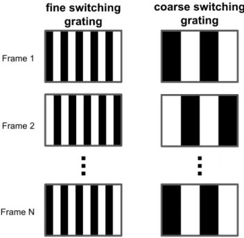
This matches our expectation based on the analysis of the neurons' responses to the changing grating stimulus. Structure of the synaptic membranes in the inner plexiform layer of the retina: A freeze-fracture study in monkeys and.

Figure 3.1: A one hidden layer ReLU network with skip connection (Eq 3.2). The nonlinearity transitions occur on hyperplanes in input space.

An identifiability theorem

Theoretical analysis

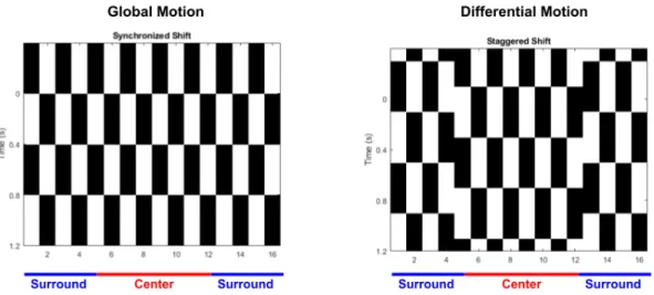
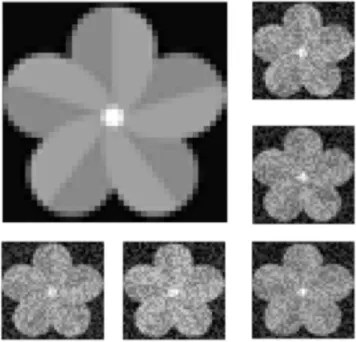
The stimulus is spatially divided between the center and the periphery of the receptive field (blue and red lines). First, the ANN was able to recover the neuron's spatial receptive field in each case.

Results II: System identification of simulated microcircuits

Simulating biologically inspired feedforward circuits

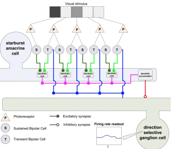
The output of the bipolar cell layer is modeled as a linear temporal or spatiotemporal inversion of a filter representing photoreceptor and bipolar cell computation with the stimulus image or video, followed by a half-wave rectifier nonlinearity (ReLU). Each amacrine cell is modeled as simply taking a linear combination of bipolar cell outputs and passing them through a ReLU nonlinearity, without further modification unless otherwise specified.

Simulating retinal circuits

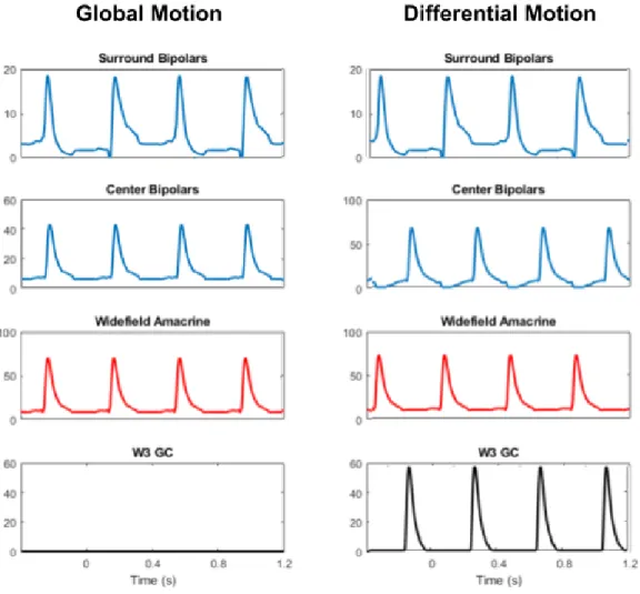
The W3 also receives lateral inhibition via wide-field amacrine cells whose receptive fields are located well outside the receptive field center of the W3 ganglion cell. The PV-5 retinal ganglion cell fires action potentials in response to the appearance of the spot in both cases, but responds strongly only to approaching movements and not to lateral movements.

Figure 4.1: Illustration of global and differential motion stimuli. In each plot, the vertical axis represents time, while the horizontal represents space

Case Study: The ON/OFF direction-selective ganglion cell

It is also hypothesized that dendritic spikes in the DSGC improve the direction selectivity of the cell [59]. Furthermore, many inhibitory pathways quickly transitioned from their random initializations to near the correct value (Fig. 4.8b, green, red). By using fewer moving point stimuli, the network could not learn the correct values ​​of the synapses of the inhibitory pathway (Fig. 4.8c).

The network on the left is pruned to one of the two candidate structures on the right. When only moving point stimuli are used to generate training data, almost all synapses are removed from the network.

Figure 4.4: Schematic of Tran model of direction selectivity. Adjacent sustained and transient bipolar cells are paired at a single segment of SAC dendrite

Implementing an “address book” constraint

Based on the stratification profile for each of the cell types, a putative connectivity matrix is ​​drawn in Figure 4.35 on the right. The trained synaptic weight matrix is ​​almost identical to the true weight matrix, the only difference is very, very little variation in the precise values ​​of the synaptic weights. The second toy retina included several cell types, specifically it also included two types of amacrine cells, modeled with ReLU output nonlinearities, which we call A1, and A2 (not in any way related to the AII amacrine cell type.) These two amacrine cell types differ in that A1 is wide-field, with a large spatial receptive field that sums over many bipolar cells, whereas A2 is narrow-field, and each amacrine cell of this type connects to only a single bipolar cell (Fig. 4.40.) IPL stratification profile for this toy retina and the putative connection matrix it gives rise to is shown in Fig.

Figure 4.33: Circuit diagram of a network with three bipolar cell types and three ganglion cell types

Study of the parametric regime in which system identification is feasible 60

Using controlled simulated settings, we conducted a systematic study to understand the dependence of successful system identification on the following factors:. i) The design of the function class 𝑓(·;W,b), and especially the presence of skip connections in the architecture. ii) The number of non-zero weights W ∈, by presetting many connections to zero. iii) Using sign constraints on the weights W∈. Figure 4.44: Left: Synaptic weight matrix for real circuit. The correct structure and weights are recovered almost perfectly, with a few differences. iv) The use ofℓ1regulation to encourage weight parsimony. v) The design of the training data set, i.e. which data refers to query. The Support Recover Score achieves perfect performance when the non-zero support (i.e., the structure) is recovered exactly.

Figure 4.43: Left: Synaptic weight matrix for true circuit. Center: Initialized synaptic weight matrix for second trained ANN

Sparsity regularization is helpful for identification of some architectures 67

When the number of free parameters is less than the number of true parameters, there is a serious breakdown in the identification of the system. System identification is much more successful and consistent when the number of free parameters is greater than or equal to the number of true parameters. When the number of free parameters is less than the number of true parameters by only 15%, there is a very large loss.

Figure 4.48: System and support recovery scores (Definitions 4.5 and 4.5) for Circuits 1, 2, 3A, and 3B respectively, using ℓ 1 -regularization and sign constraints.

The four subtypes of the alpha ganglion cell

Data collection using multi-electrode array

The stereotyped response of each neuron to repetitions of the same stimulus helps keep track of the neuron's health throughout the duration of the recording.

Data preprocessing

The retina is positioned so that the ganglion cell layer is aligned with the array of electrodes.

A system identification problem for alpha cell circuitry

Structurally analogous to circuits 3A and 3B in Figure e), the ANN is initialized to include all components and connections used in all four hypotheses. f) Estimates of structure recovery and support when the ANN in (e) is trained on data generated by simulated circuits with architecture matching (a)-(d). In our case, the size of the sOFF𝛼subunit was approximately 150𝜇m (Figure 5.4 top left), while the size of the tOFF𝛼subunit was approximately 95𝜇m (Figure 5.5). The sOFF𝛼 cell can also use a push-pull type model involving rectified subunits, but these subunits are inhibited by another set of subunits with the opposite polarity via the amacrine cell (Fig. 5.3d.).

Figure 5.2: Contrast-reversing grating stimulus

Fitting an ANN to alpha cell data

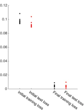
This serves as a “floor” to better contextualize the system of the trained ANNs.

Recovery of known biological information about the alpha cell

Proportion of variance in retinal data explained by trained ANN separated by cell type. The spatiotemporal filters of the bipolar cell subunits in each trained ANN correctly reflected the persistent or transient and OFF or ON properties of each neuron. Thus, the ANN successfully recovered known information about each of the four alpha cell circuit subtypes.

Figure 5.7: Left: Example of quality of fit to ganglion cell firing rate. Right:

The ANN correctly identifies the circuitry of the transient OFF alpha

All four synapse types remained in the final trained ANN for all four alpha cell subtypes (Figure 5.13). In the case of the transient OFF subtype, this finding confirms something that has already been elucidated by painstaking attempts to dissect the biological circuit [58]. In the trained ANN, there are linear bipolar cells that also excite the ganglion cell.

Figure 5.12: Ratio of magnitude of second peak to first peak in each set of learned temporal filters for linear bipolar cells in the trained ANNs, separated by cell type.

System identification as a tool for hypothesis selection

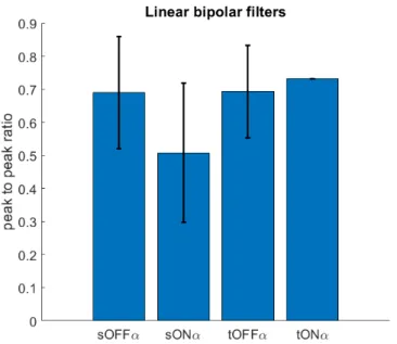
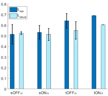
𝐿sys and 𝐿supp (Eqs. 5.1 & 5.2) for artificial neural networks trained on data sets recorded from each of the four types of alpha ganglion cells in the rat retina. Thus, in all four subtypes, the contribution of linear subunits is greater than that of nonlinear subunits. We should also note that our study was underpowered in all subtypes except the tOFF𝛼 cell which was overrepresented in the data set and accounted for 2/3 of the cells studied.

Figure 5.14: Comparing the strength of linear and nonlinear pathways in the learned alpha cell models

Summary

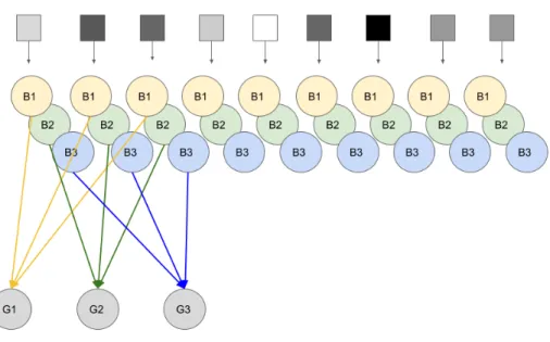
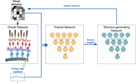
The stimulus generating network receives an approximation of the structure and weight of the network from the trained ANN. The bipolar cells convolved the stimulus video with a temporal filter and passed the output through a ReLU nonlinearity. This may explain the failure of the algorithm to perfectly recover the synaptic weights of the circuit.

Figure 6.1: Cartoon demonstrating stimulus generation method. If a flower is given as the seed stimulus, taking random steps in stimulus space will give rise to several noisy-looking pictures of the same flower.

Results IV: An exploration of algorithms for input selection in

An adversarial stimulus generation algorithm

An algorithm to select between two classes of stimuli

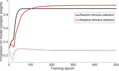
We applied this algorithm to the stimulus distribution 𝐴 that contained both random flickering and moving random pattern stimuli equally. Each new set of stimuli, 𝐵𝑖, is composed of some moving stimuli with a random pattern and some random flickering stimuli, and the ratio of these depends on which stimuli cause the largest error in this phase of training. We found that early in the structure learning phase, the algorithm prefers moving random pattern stimuli over random flickering stimuli (80% motion stimuli). During the "fine tuning".

Figure 6.3: Projection score over the course of training for two trained ANNs with different training algorithms

An algorithm to maximize output of the circuit

We then perform backpropagation from the output of the stimulus generation network all the way to the stimulus (Figure 6.6). Thus, we can calculate the partial derivative of the network output with respect to the stimulus image and use the gradient ascent to. Since the algorithm was quite complex, we wanted to start very small to understand the behavior of the algorithm. This is intuitively a very simple stimulus to choose if we want to increase the firing of the ganglion cell in Fig.

Figure 6.5: Schematic of the active stimulus-generation algorithm.

An algorithm for optimal stimulus design given competing circuit

However, because there was no mechanism to encourage the algorithm to maintain diversity in the stimulus set, as the stimulus-generating network converges to this high-contrast "checkerboard" stimulus, the stimulus groups used to train the trained network become very monotonous. Initialize an ANN whose output is the squared difference between the output of network A and that of network B (Fig. 6.11).

Summary

Within this work we have mentioned gene circuits as a possible target, but another logical next step would be to move one synapse down the visual system, and apply this technique to neurons in superficial superior colliculus or lateral geniculate nucleus. As mentioned in the introduction, this technique is applicable to any feedforward circuit for which partial prior knowledge exists and whose input and output are easily accessible. Intersectional strategies for targeting amacrine and ganglion cell types in the mouse retina, August 2018.

Conclusion and future directions