Total atmospheric opacity of the 1\lartic atmosphere at lJlm can be derived from the 1\IOLA refiectivit:-.· measurement. Comparison of the .t--.10LA-derived opacity~' with the TES-derived opacity ~· yields information on the aerosol particle size distribution.
List of Figures
59 Gl 62 6-l 66 3.9 l\IOLA instrument model output for two different cloud structures 6 3.10 Comparison of TES brightness temperature data with l\IOLA.
List of Tables
Chapter 1 Introduction
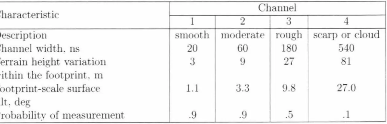
- Description of the MOLA instrument
Reflectivity measurements allow us to calculate total atmospheric opacity or calculate surface albedos. General description of the :\IOLA-1 laser and scientific objectives can be found in Zuber et al.
Time
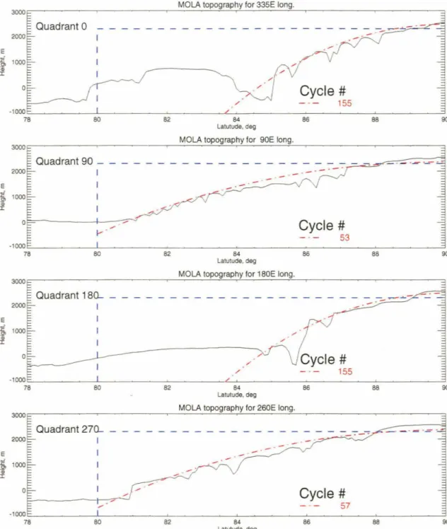
- Topograph y of t h e polar re g ions
- Observations of the polar clouds
- Interpretation of the reflectivity
- Atmospheric opacity
- Surface albedo
- Summary
- Introduction
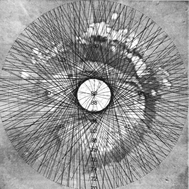
- Topography data
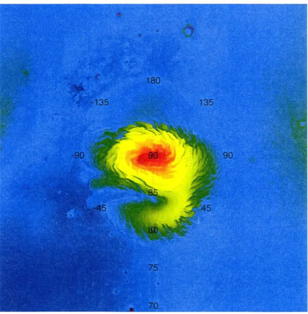
The composition of the ice caps was determined by the Viking Infrared Thermal _ Iapper (IRTI\I). The detailed shape of the 1\north polar ice cap (-·pre) has been measured with high precision by the I\Iars Orbiter La<>er Altimeter (I\IOLA) instrument on the l\Iars Global Surveyor (I\IGS ).
Elevation , m
Elevation, m
Sublimation model
If the partial pressure of water vapor, PH2o(t), is greater than Psat(T), then water condensation occurs on the surface and the cap increases. The water loss during the new year is then multiplied b~· 10 and the shape of the cap adjusted to a function of latitude.
Timescales
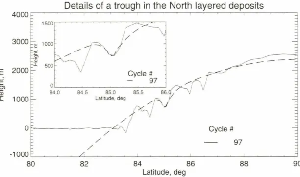
Comparisons of the modeled ice sheet and trough with ~lOLA topographer~· profiles are discussed in Section 2.5. 23. See section 2.4 for a discussion of the time scale. which slows down sublimation relative to ice or vacuum conditions.
Results
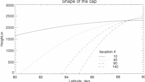
- General form of the ice cap
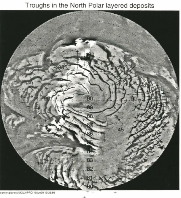
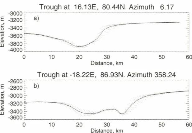
- Form of the t roughs
We stopped confining the model when the simulated profile matched the measured shape of the ice sheet. The lOOm from the bottom of the trough is bowl-shaped, with almost equal slopes on both sides.
Shape of the South Pole Layered Deposits
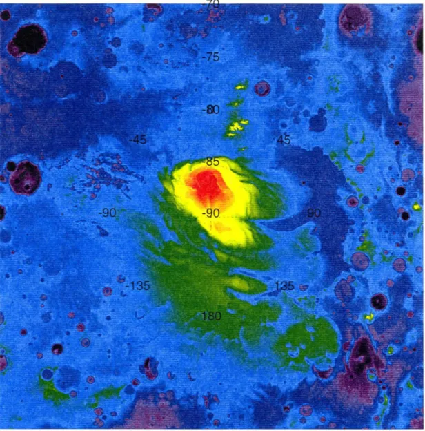
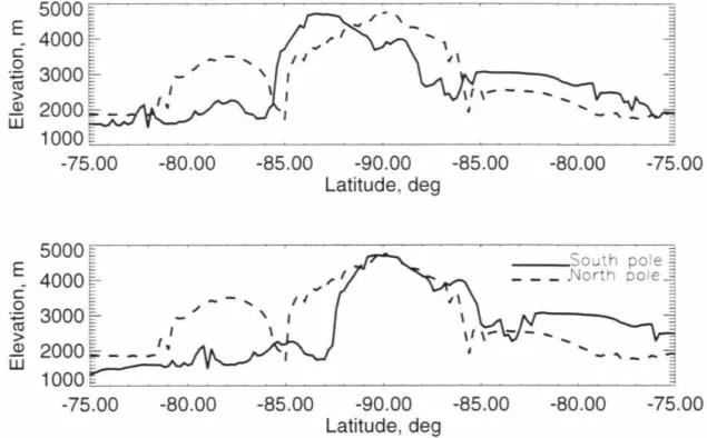
The top panel shows the relative shift (~3 degrees) of the topography maximum of the South Pole cap relative to the true pole. Because the 'PIC and the South Polar Layered Deposits (SPLD) are similar in size and shape. We know that the thermal inertia of the surface layer of the SPLD is low.
2. 7 Discussion
Conclusions
In this paper, we present the results of an ice sublimation model from the surface of the northern 1\Iartic ice sheet and compare them with the shape of the ice sheet observed by f\IOLA. The combined effect of all three processes on the shape of the cap has not yet been investigated. You were able to delineate the time scale for the formation of the ice sheet (using values measured on Earth) somewhere between 5 - 100 million years.
Appendix 2.1
Convection of the water vapor
Chapter 3 Polar night clouds
- Int roduct ion
- Previous work
- Instrument description
- Observations
- North Polar Region
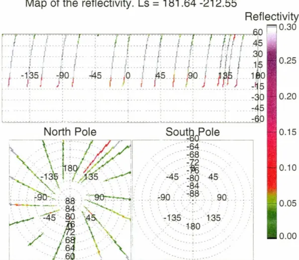
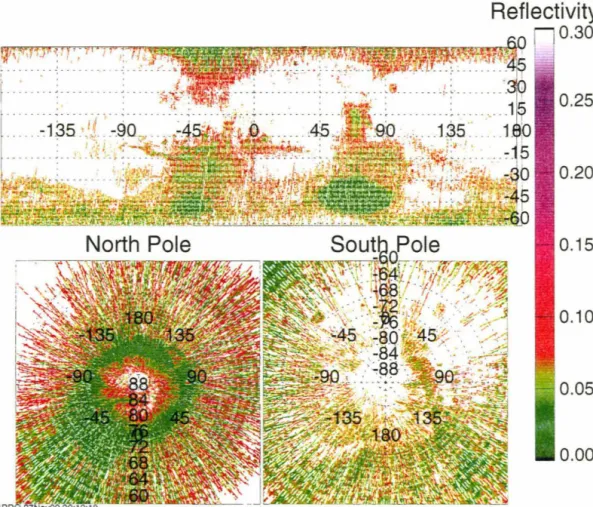
The most extensive cloud formations were observed over the orth-polar ice cap at the end of the northern winter (Ls. They exhibit the same structure and reflective properties as clouds, observed at the end of the northern winter. In the following sections we detail observations of the clouds for northern and southern polar regions separately.
Fine details of the clouds
South Polar Region
Such an orbit provided much more extensive temporal coverage of the South Pole, compared to the North Pole coverage, where MOLA only passed once in 12 hours. We can separate cloud structures or patterns observed over the South Pole into two types. They do not show as clear cloud tops as the clouds over the remaining caps, but spread from the ground to about 7 km heights above the ground.
Cloud opacities
).lOLA reflectance data could be used to estimate the optical density of northern polar clouds. MOLA received the unsaturated return from the ground through the cloud cover above the ice cap. We could not obtain unsaturated reflectance measurements in the south polar region.
Model
- Cloud reflections
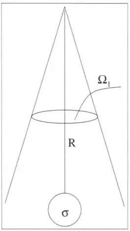
R is the range of the laser to a particle and (j is the scattering cross section of a particle. This cross section can be calculated using the particle size distribution formulation (Hansen and TraYis (1974)). Shape of the Earth's return cirrus clouds can be used as an analogue to the l'dartian cloud return.
SLA02 Waveforms
Vertical distance, m
Backscattering coefficient
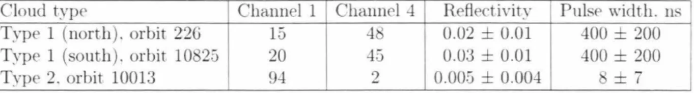
This indicates high values of particle number density gradients right at the top of the clouds. The best explanation for type 2 clouds is patches of nascent C02 clouds on a scale of about 200 m each. The average values of the backscatter coefficients were calculated for each of the tracks and are shown in Table 3.4.
3. 7 Comparison with the TES polar night data
Discussion
Occasionally, MOLA has recorded cloud reflections at night in locations outside the polar regions of the planet. We need to investigate the contribution of radiation and adiabatic cooling to the process of cloud formation. In light of the l\lGS cloud observations and recent radiation balance modeling b~· Forget et al.
Conclusions
It is not possible to calculate the mean particle size from measurements of the backscattering coefficient .:\lOLA alone. A microphysical model of C02 crystal formation is required to obtain information about particle sizes and number densities. The :\-IGS Radio Science temperature pressure profiles will provide us with more insight into the radiative properties of clouds and the conditions of cloud formation.
Chapter 4 Reflectivity observations in the MOLA investigation
- Introduction
It is affected by the underlying terrain albedo (A) and extinction of the E' photons from the laser beam by atmospheric aerosols and can be expressed as R = A* e-'2T. You will present a method for calculating the aerosol scale height using the reflectance data in section 4. The method is based on an analysis of the total atmospheric opacity as a function of elevation.
4. 2 Available datasets on albedo and opacity of Mars
Albedo
To calculate the atmospheric opacity (section 4.5) we used the albedo dataset constructed by Plescot and l\liner (19 1) from the IRTI\1 measurements.
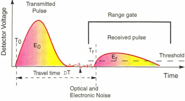
MOLA reflectivity
The received optical pulse energy Er (in joules) can be calculated by dividing the area of the received pulse (A. voltsxns) by the responsivity of the detector assembly (Rdet. volts/watt). The surface T\·lOLA footprint is about 100 m in diameter for the map configuration (;=::: 400 km altitude). It was changing during the abort and science phase orbits due to the elliptical nature of the orbit.
Pathfinder site
These tracks largely cover the Northern Hemisphere and spread uniformly in longitude. This makes it possible to estimate the maximum albedo of l\Iars w<:> that can be expected at these wavelengths. The saturation problem limited our initial coverage to the regions with very low albedos, such as the Arctic dunes.
Reflectivity
Most of the reflectance data are saturated because the laser energy reaches maximum output during the mission and the atmosphere is very clear. These data were collected after the threshold of the channel 1 detector was raised to the maximum value. The primary objective of the reflectivity measurement in the MOLA survey is to compile the global map of normal albedo on Mars at 1,064J.Lm wavelength.
Reflecti vity
Low reflectance values in the Southern Hemisphere are likely due to turbidity created by the sublimation of the seasonal ice sheet.
Reflectivi ty
Ve will demonstrate calculation of :\lOLA albedo using atmospheric opaci(v simultane!~· measured by the TES instrument. The increase in the returned signal amplitude due to the opposition effect for the l\IOLA measurement on l\lars is not known accurately The scaling of the dust opacity in the infrared with respect to the I\IOLA wavelength is very important for the determination of albedo.
The deviations from the ratio during the mapping mission can be illustrated by comparing 9J1m opaque~· with the Y\10LA 1J1111 opaque~··. The high Yalues ratio is due to improvement in small submicron particles in the atmosphere relative to the dust storm season period. I assume that the dust is the only scattering aerosol in the atmosphere during this time.
Syrtus Major Albedos Comparison
Calculation of atmospheric opacity
- Corre ctions
Plescot and f\Iiner (1981) state that they used the clearest period of the f\Iartian atmosphere to compile the data set. We hope to be able to compile an albedo map from the !\lOLA reflectance measurement and use it as the base map of darkness calculations. The low phase angle allows us to minimize the effects of dust forward scattering on the images.

Examples of opacity calculations
We did not use images with high phase angles (> 50°) to avoid brighter surface albedo of aerosols and surface phase function effects. This is consistent with spectroscopic observations of the average Martian surface in visible and infrared wavelengths (Soderblom (1992)), as well as with recently published composite spectra of Mars by Erard and Calvin (1997). Surface albedo for both regions was taken from the Plescot and Miner (1981) data set and corrected to the MOLA wavelength using equation 4.6.
MOLA and VL2 Daytime Opacity
The Mars Pathfinder Lander (Smith and Lemmon (1999)) made observations of atmospheric turbidity at several wavelengths, including 986 nm, which is very close to the MOLA wavelength. Extinction efficiencies for the Viking Landers, Pathfinder, and MOLA wavelengths do not differ significantly based on the particle size distribution that exists on Mars. Due to the characteristics of the MGS orbit, we could not fly over the same area in one or two days.
4. 7 Scale height calculation
The Syrtus Major opacity only begins to rise when the dust storm season begins, i.e. around Ls = 220°. They concluded that opacity at this wavelength is similar to that reported by the Viking Landers.
MOLA Day time vs. Night time Opacity
MOLA Opacity. Polar regions
Oly mpus Mons
At the beginning of the mapping orbits (Ls = 103°), MOLA returned a significant amount of unsaturated returns across Olympus Mons. Perhaps the cause of the darkness is the bands of clouds during the day, which form during the summer. It is likely that the equatorial band of clouds existed before the start of the mapping campaign.
Alba Patera
4. 7.3 Hellas Basin
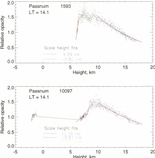
The negative scale heights below 6km height possibly correspond to an inversion layer in the atmosphere or the edge of the cloudy region. For example, opacity variation with height for lane 339 best fits scale heights of. Optical density of the atmosphere near the edge of the Hellas basin does not depend on the time of day, and this is mostly due to the dust particles suspended in the atmosphere.
Opacity change with height over the Hellas Basin
Hellas Scale Heights
Opacity in Valles Mariner is
Using the Viking Color MDIM (sequence 583a) as described above to correct the albedos of the canyon floor and walls, we were able to estimate the opacity over the canyons. It can be seen from the figure that the turbidity inside the canyons is higher than the turbidity at the top, apparently due to atmospheric aerosols inside the canyons. The linear nature of the fit to the data suggests that N(z) and k~:(::.) are approximately constants.
Opacity vs. depth and pressure
Depth of the canyon , km
Opacity "events"
The Hubble Space Telescope team reported observations of the water mist earlier in the season (Lee eta!. Th<:> local time for the I\IOLA observations was about 5:00 p.m. and the sun was about to set. The suggested explanation is that photon extinction is due to condensed water or C02 ice clouds near the North Polar Vortex.

Summary
Comparisons of the lpm turbidity results with the 9pm TES turbidity will add further to our knowledge of eli particle size, distribution in the :-.lartian atmosphere'.
Acknowledgments
Chapter 5 Summary and future research
- Sublimation of the ice caps
With this model we studied the change of shape of the ice caps under simple assumptions. The inferred time scale for the formation of the observed shape is significant!~· greater than any of the known orbital Yariations. An ice flow model is needed to understand the evolution of the ice caps for periods longer than 100 million years.
Albedo and opacity
Calculated values of the total atmospheric opacity are similar to the opacity values performed at the Viking Lander stations (Colburn et al. Observations of the scale height of the aphelion water cloud belt o\·er Ol~··mpus l\lons are consistent with the atmospheric scale height One of the primary scientific objectives of the l\IOLA survey is to compile a map of normal surface albedo at the ).lOLA wavelength.
Conclusions
In Section 4.4 we discussed an algorithm that uses the 9J1m~· dust obscurity. derived from MGS thermal emission spectrometer observations by Smith et al. 1999b) and presented some initial results. The albedo values at the !\lOLA wavelength appear to be consistent with the Plescot and :--.liner (1981) data set.
Bibliography
The role of sublimation in the formation of the northern ice sheet: results from the Tlw l\Iars Orbiter Laser Altimeter. Thermal and albedo mapping of the polar regions of l\lars using Viking Thermal l\lapper observations .1. Thermal and albedo mapping of the polar regions of l\1ars using Viking Thermal Mapper observations .2.