Introduction
Scope of the Thesis
Crystallographic defects and impurities in solid-state materials typically control charge transport at low temperatures and in highly disordered materials due to the interactions between defects and charge carriers [1,2]. In addition, magnetic impurities or defects in the presence of spin-orbit coupling can rotate or reverse the spin of charge carriers and thus control their spin relaxation, a quantity of key interest in spintronics and spin-qubits [13–15], while line defects can filter electrons with opposite valleys in valleytronics [16].
Theoretical Tools for Electron-Defect Interaction
The carrier mobility or electrical resistivity in metals is typically calculated using the phase shifts of the partial waves around the impurities [25]. The starting point for the self-consistent calculation is a given potential, whose detailed form is unimportant, with a suitable parameter - e.g. the potential depth in the square-well model.
First-Principles Methods for Electron-Defect Interaction
The atomistic details of the short-range potential and the atomic relaxation around the defect play a key role and cannot be captured by simplified models. Although Bloch modes are an appropriate representation and the eigenmodes of the Hamiltonians are used in electronic structure calculations, other representations are available, such as Wannier functions (WFs).

Outline of the Thesis
The spatial decay of the matrix elements in the WF basis is critical to the accuracy of our approach. Our formalism uses only the wave functions of the primitive cell and can efficiently compute matrix elements.
Efficient First-Principles Method for Computing Electron-Defect
Introduction
Ab initio e-d calculations can benefit from existing tools developed for electron-phonon (e-ph) interactions, which allow accurate calculations of relaxation times (RTs) [2-5], matrix elements and their interpolation [6]. and phonon-limited carrier mobility [7–. Using our approach, we can calculate and converge the matrix elements and their associated RTs and defect-limited carrier mobility.
Derivation of an Efficient Formalism for Electron-Defect Interaction 15
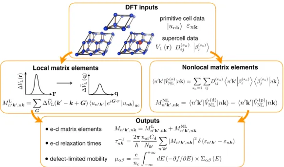
The local and non-local potentials of the KS potentials can be calculated in the pristine and the defect-containing supercells using standard DFT calculations. Here we develop a new approach to reduce the computational cost of the local and non-local matrix elements.
Electron-Defect Interaction Workflow and Computational Details
We include the nonlocal matrix elements here because they can affect the phase and magnitude of the total matrix elements Mmn(k0,k). Once calculated, the e-d matrix elements are used to calculate ee-d RTs and defect-limited mobility, among other quantities of interest.
Comparison between the All-Supercell Method and Our Approach . 20
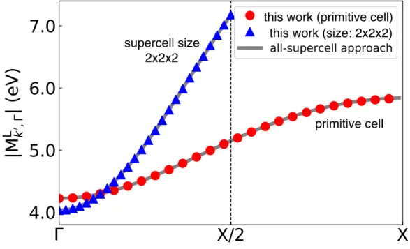
Hence, computing the local matrix elements in a uniform BZ grid with Nk points has a cost of order Nat3 in our method, versus a cost of Nk × Nat3 in the all-supercell method. The initial state for the local matrix elements is in the lowest valence band in Γ, and the final states are in the same band with crystal moment k0 along the Γ−X line of high symmetry.
Rigorous Strategy for Converging Electron-Defect Relaxation Times 26
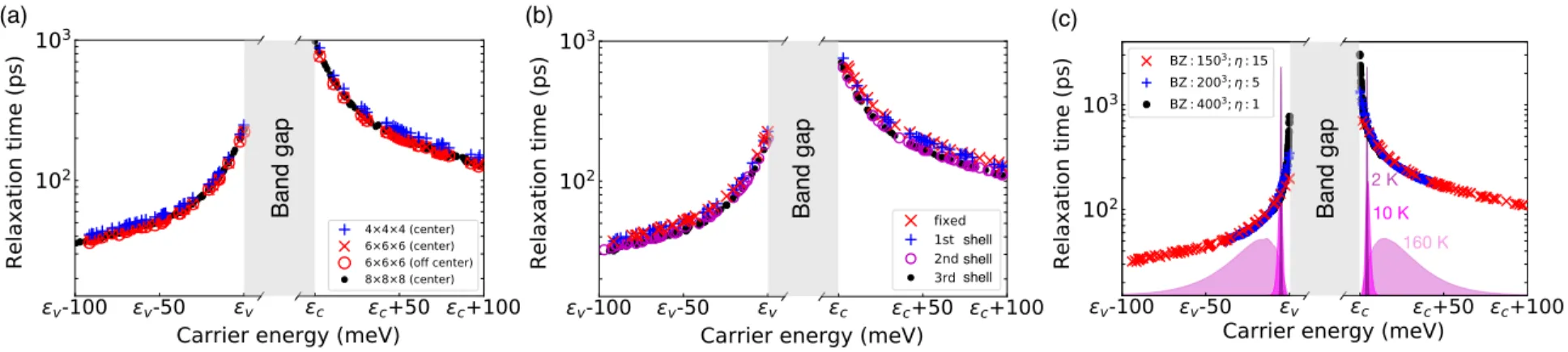
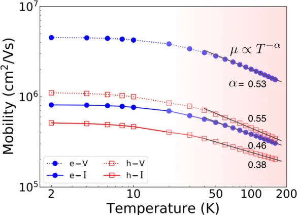
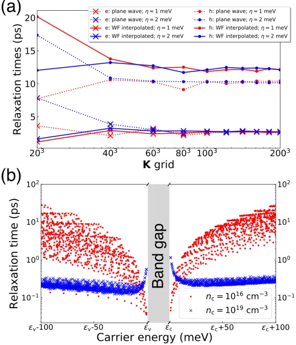
Figure 2.4(c) shows the RT for several values of the energy spread η and gives the corresponding grid BZ at convergence. To estimate the range of carrier energy that contributes significantly to mobility, we plot the integrand of the mobility formula in Eq. As the temperature increases, the peak of the function broadens and moves away in energy from the band edges, indicating that the energy region contributing to mobility shifts to higher carrier energies.
Summary
The development of such a fore-d matrix element interpolation method is the main goal of the next chapter. However, for charged ti-d defects the matrix elements in the Wannier basis do not decay fast enough in real space due to the long-range nature of the examined Coulomb potential. Using the wave functions and the screened Coulomb potential, the e-d matrix elements on the coarse BZ kc-grid are calculated.
Ab Initio Electron-Defect Interactions Using Wannier Functions . 33
Derivation of a Fourier-Wannier Interpolation Scheme for Electron-
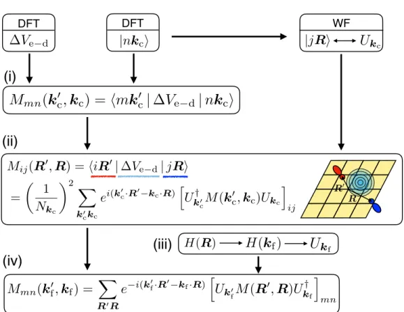
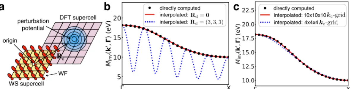
Consequently, to calculate the e-d matrix elements in the Wannier representation, only a small number of grid vectors R are needed, which are arranged in the WS supercell centered at the origin. The e-d matrix elements in the Wannier representation can be written as a generalized double Fourier transform of the matrix elements in the Bloch representation, which are first calculated on a coarse BZ grid with kc: points. Note that the oure-d matrix elements in the Wannier representation require WF only for the primitive cell, while the method developed in Ref.
Wannier Interpolation Workflow and Computational Details
U
Validation of the Wannier-Fourier Interpolation Method for Electron-
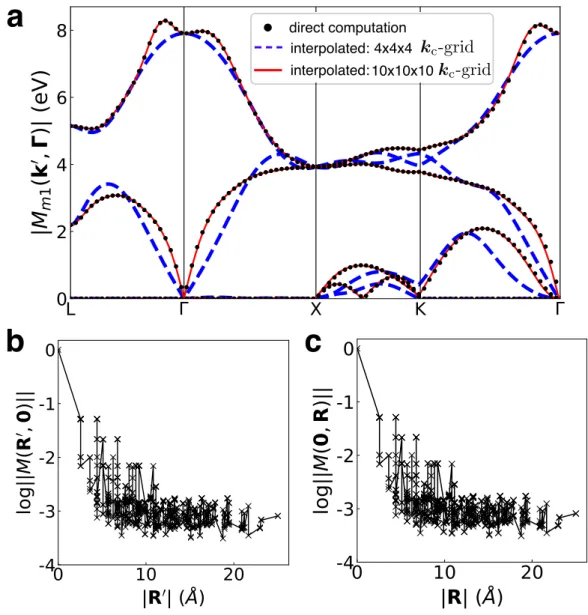
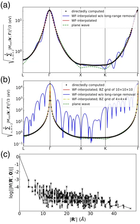
Briefly, we compute the matrix elements of the coarse-d grid using primitive cell wave functions and obtain the perturbation potential due to the vacancy defect using a 6 × 6 × 6 supercell with a 2 × 2 × 2 k-point grid. The data are for a neutral vacancy in silicon, with the d-matrix elements calculated for the four lowest valence bands and along the high-symmetry BZ lines L–Γ–X–K–Γ shown in Figure 3.2. To analyze the spatial behavior of the matrix elements in the WF database, we define for each pair of grid vectors R0 and R the maximum absolute value of ti-d matrix elements as ||M(R0,R)|| =maxi j|Mi j(R0,R)|.
Carrier Relaxation Time and Mobility Using the Wannier Interpola-
We find that the matrix elements in the WF basis decay exponentially within a few unit cells, confirming that the WFs are a suitable basis set for the interpolation of e-d matrix elements. Number of points k
Speedup of the Wannier Interpolation Method Compared to the Di-
Wannier Interpolation Method for the Brillouin Zone Summation in
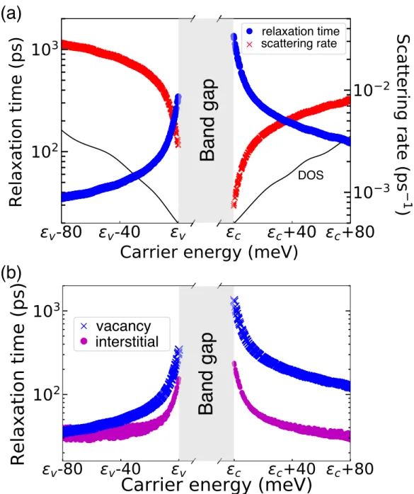
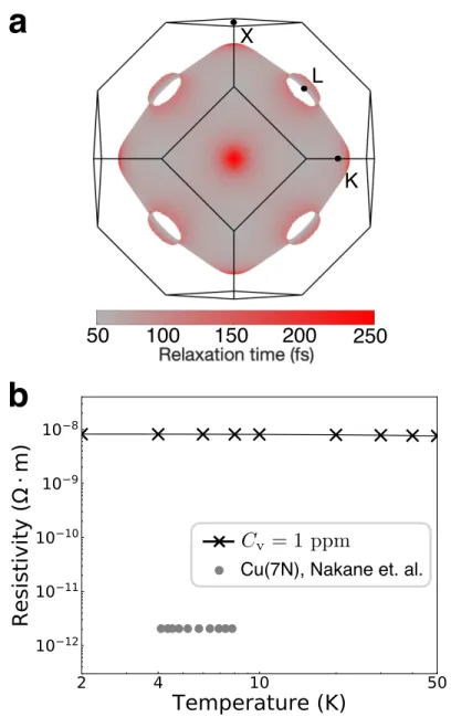
For copper, we show the scattering strength for electronic states within 50 meV of the Fermi energy εF, and in silicon for states within 100 meV of the valence band maximum. The e-d RTs due to the distribution of vacancies in copper are highly dependent on the state - we find values of Our method can predict a lower limit of residual resistance due to intrinsic defects in an ideally pure material.
Summary
Subsequently, the long-range part of the e-d matrix elements is removed, while the short-range part is transformed from the Bloch mode to the WF basis using the unit matrices U(kc). The short-range part of the e-d matrix elements of the WF basis is used to interpolate any short-range part of the e-d matrix elements of the Bloch modes on a finekf grid. In step 3, we compute the local and non-local d matrix elements using the property of the complex conjugate of the matrix elements.
Ab Initio Electron-Defect Interactions for Ionized Impurities in
Introduction
As previously discussed, these are the two essential steps to calculate the defect-limited carrier mobility. The e-d matrix elements are usually calculated using plane waves instead of Bloch waves as a simplifying assumption [17]. In this work, we aim to develop methods to calculate and interpolate your d matrix elements due to ionized impurity scattering.
Electron-Defect Matrix Elements for Ionized Impurities
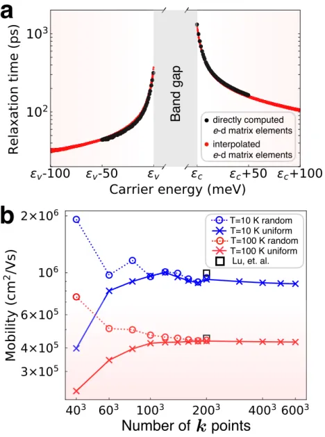
In some cases, the curve for the ab initio e-d RTs as a function of carrier energy is the best fit of the unconverged e-d RTs [22]. A relevant example is the long-range Frohlich interaction in polar materials, which is added to the momentum space in the workflow of e-ph calculations [23–25]. V˜(|k0− k−G|) humk0|e−iG·r|unkiuc, (4.4) where |nki is the Bloch state with a band index n and a crystal moment k, G is the reciprocal lattice vectors of cells primitive, and unk is the periodic part of the Bloch wave function |nki.
Wannier Interpolation Method for Charged Defects
To overcome this challenge, we use a smooth phase approximation to remove the so-called long-range part of the Coulomb potential screened by the e-d matrix elements before performing the double Fourier transform in Eq. The long-range part of thee-d matrix element in the coarse grid BZ kc is defined as. 4.13). The remainder of thee-d matrix elements, after the long-range part is removed, is defined as the short-range part of the thee-d matrix elements.
Workflow and Computation Details
Electron-Defect Matrix Elements for Charged Defects
However, after removing the long-range part in the interpolation procedure, the interpolated matrix elements successfully reproduce the directly calculated results. Similar to the previous case, the interpolated matrix elements without removing the long-range part cannot reproduce the directly calculated results. After removing the long-range part, the interpolated matrix elements actually reproduce the directly calculated results.
Electron-Defect Relaxation Times due to Charged Defects
The plane wave matrix elements can reproduce the matrix elements well around the Γ point similar to the previous case. For example, electron RTs using WF interpolation converge to the same value for two different expansion values when using a dense BZ grid with more than 1 million kf-points. RTs calculated using plane waves also converge to the same RT value because there is only one band (lowest conduction band) for the electron while interband dispersions are.
Electron Carrier Mobility as a Function of Doping Concentration in
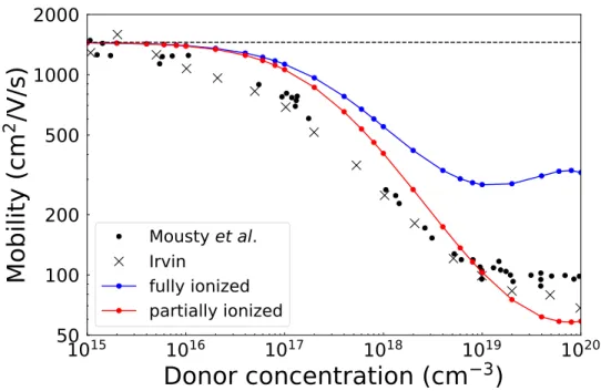
For the fully ionized case, the electron carrier mobility does not agree well with experiment, especially at higher doping concentrations. Future work will further investigate the deviation of the calculated carrier mobility from the experimental data. Future work on charged defect will also include e-ph scattering to obtain a more accurate temperature dependence of the carrier mobility.
Summary
All MPI processes work at the plane wave parallelization level of the QE subroutines. FFT grid elements (dfftp%nnr) are allocated and distributed between MPI processes. Suppose we want to obtain the Fourier coefficients of the perturbation potential for the wave vectors nqc.
The PERTURBO Open Source Code and its Electron-Defect
Introduction
During my PhD work I was involved in the development and testing of parts of the PERTURBO code and I am currently working on incorporating the electronic error (e-d) routines into the code to make them available to the community. This step would dramatically increase the impact of the work discussed in this thesis, as different research groups will be able to apply and extend the methods developed in this thesis. In this chapter, we discuss how to integrate all calculations of initial electronic errors (e-d) with the current PERTURBO code.
Boltzmann Transport Equation for Electron-Defect Scattering
When Fnk was calculated either within the RTA or by iteratively solving the BTE in Eq. 5.8), we get the conductivity tensor as The Ti-d relaxation times calculated in previous chapters are based on RTA rather than an iterative approach. Using the interpolation methods for neutral and charged defects developed in this work, the defect-limited mobility or the mobility in the presence of e-ph and e-d interactions can be calculated.
Software to Compute Electron-Defect Matrix Elements for Neutral
Using the Wannier basis, the matrix elements can be interpolated for each momentum pair on a fine BZ kf grid. The methods for interpolating the e-d matrix elements using Wannier functions for neutral defects and charged defects are described in Chapters 3 and 4 respectively. The resulting e-d matrix elements are used to calculate the e-d RTs due to elastic scattering within the lowest-Born approximation in Eq.
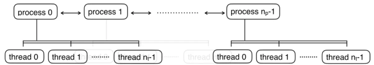
Parallelization of Electron-Defect Scattering Calculations
In MPI routines, Gvectors and corresponding coefficients are shared and distributed between MPI processes. After computation, we use the parallel subroutine QE to collect and transmit the Fourier coefficients between the MPI processes. After all distribution rates are calculated, we use the QE byproduct to collect them from all MPI processes.
Summary
The third method developed in Chapter 4 is a Wannier interpolation method for para-d matrix elements for charged defects that correctly accounts for the long-range nature of the perturbation potential. Ve−d(r− ri), (A.4) where ∆Ve−d(r − ri) denotes the perturbation potential due to a defect located at ri, and we consider non-interacting defects of the same type. If a general atomic position τs is chosen, the Fourier coefficient B(s)jk (q) becomes, using the properties of Fourier transforms, C.4) The scalar product in Eq.
Future Extension of ab initio electron-defect interactions