Article
Urban Land Allocation Model of Territorial Expansion by Urban Planners and
Housing Developers
Carolina Cantergiani * ID and Montserrat Gómez Delgado ID
Department of Geology, Geography, and Environment, University of Alcala; 28801 Alcaláde Henares, Spain;
* Correspondence: [email protected]; Tel.: +34-91-885-5263
Received: 21 September 2017; Accepted: 27 December 2017; Published: 29 December 2017
Abstract: Agent-based models have recently been proposed as potential tools to support urban planning due to their capacity to simulate complex behaviors. The complexity of the urban development process arises from strong interactions between various components driven by different agents. AMEBA (agent-based model for the evolution of urban areas) is a prototype of an exploratory, spatial, agent-based model that considers the main agents involved in the urban development process (urban planners, developers, and the population). The prototype consists of three submodels (one for each agent) that have been developed independently and present the same structure. However, the first two are based on a land use allocation technique, and the last one, as well as their integration, on an agent-based model approach. This paper describes the conceptualization and performance of the submodels that represent urban planners and developers, who are the agents responsible for officially launching expansion and defining the spatial allocation of urban land. The prototype was tested in theCorredor del Henares(an urban–industrial area in the Region of Madrid, Spain), but is sufficiently flexible to be adapted to other study areas and generate different future urban growth contexts. The results demonstrate that this combination of agents can be used to explore various policy-relevant research questions, including urban system interactions in adverse political and socioeconomic scenarios.
Keywords: urban land allocation model; agent-based model; spatial simulation of urban growth;
urban planners; developers; urban modeling
1. Introduction
Urban growth is considered a complex phenomenon due to the strong interactions between different economic, social, environmental, cultural, and institutional components. A deeper understanding of how, why, and where these interactions occur is required in order to be able to plan the territory and create better futures for a constantly growing population. Thus, urban planning is fundamental, as is the need to comprehend and anticipate territorial changes. Modeling offers an alternative means to achieve this due to its capacity to create different possible future scenarios and depict the consequences of urban growth [1–3].
Recent decades have witnessed exponential growth in the use of exploratory models based on different techniques (e.g., stochastic, artificial intelligence, and fuzzy tolerance) in the field of simulation. Although cellular automata (CA) predominate [2], agent-based models (ABM) open new perspectives. Both were originally developed in the field of artificial intelligence with the aim of reproducing the knowledge and reasoning of several heterogeneous agents with the capacity for autonomous action in a specific environment, who at the same time need to coordinate to jointly solve planning problems [4].
Environments 2018,5, 5; doi:10.3390/environments5010005 www.mdpi.com/journal/environments
Environments 2018,5, 5 2 of 21
However, the use of modeling as a tool to support urban planning has remained limited due to historical skepticism about modeling designed for this purpose [5–7]. Nevertheless, although few ABMs have been employed to address urban issues, other cellular models such as CA have gained more widespread acceptance [8–11]. This is confirmed in a review of urban simulation modeling techniques by Triantakonstantis and Mountrakis [2], who found that more than 80% of the publications analyzed had used a CA, whereas ABM only accounted for less than 10%. These statistics must be placed in context, since CAs have a long history of being used for spatial modeling, whereas ABM are comparatively new in this field. Nevertheless, CAs pose some problems, for example when considering long distance interactions [3], thus paving the way for the use of ABM in the urban modeling arena.
ABM techniques are particularly suitable in this field to gain a better understanding of the urban development process because they allow individual simulation of each agents’ behavior and show how, in conjunction, their behavior produces changes in the territory in the form of urban growth.
Hence, ABM provides a good laboratory for developing new models of cities, since they elucidate how different city elements interact and thus enable planners to better understand what might happen in the future [3,12,13].
Another important issue to consider is the geographical scope of urban ABM, which varies according to purpose and encompasses multiple spatial scales, although always considering individual behavior. Thus, the literature contains models aimed at exploring local issues such as residential mobility [14] or emergency situations [3,15], and others with a broader, regional scope, for example those aimed at determining urban segregation or informal settlement formation [16–19]. Most have been designed to simulate housing and land market dynamics [20–27]. Consequently, the application of ABM has proved very versatile at different scales, including the sub-regional scale, here understood as the geographical level between the municipal and regional scale.
The sub-regional scale is particularly suitable for urban planning, since urban growth and its impacts can be better controlled at this level. This is especially useful in Spain, where planning is legally proposed at municipal level, with few examples at regional scale [28]; however, it is at this latter level where not only urban growth phenomena but also their territorial, environmental, and other associated impacts could be managed more efficiently. The lack of legal instruments at sub-regional scale has created serious problems, especially during the recent real estate boom [29–31].
Besides scale, a further advantage of ABM when simulating urban growth processes is their capacity to reproduce the behavior, actions, and interactions of the multiple agents involved, who may present diverse profiles (e.g., social, political, and economic). Urban planners and developers are unquestionably among the most important agents in urban growth, since they decide the amount of land to be converted to urban uses, as well as where development should first take place.
The population represents another important agent in this process, since the population’s behavior is responsible for the demand for new housing, in this case occupying the available dwellings generated by the two abovementioned agents.
Implementing an ABM that simultaneously considers both policy-making and the residential development process poses an enormous challenge in modeling due to the large number of variables to consider (accounting for both internal status and externalities), the spatial (sub-regional) and temporal scale (behavior may occur at different time intervals), and above all, the combination of top-down and bottom-up approaches. With respect to the spatial and temporal scale, it is assumed that these are strictly linked to the kind of data used. Many models developed to study changes observed at the urban level consider stylized data in a hypothetical world. Artificial cities and rules are constantly being created in order to test these models and their underlying theories [21,22,26,32].
Although some independent allocation models have been used to simultaneously simulate both levels of the planning process (policy-making by urban planners and residential expansion by developers), only a few ABMs have been aimed at considering both when simulating urban growth at the sub-regional scale [33–35]. Some of these have considered the environment or urban planners as agents, albeit not with the same goal [18,20,36,37]. In contrast, many urban ABMs consider
developers as agents, mostly focusing on land market dynamics [21–23,32]. Similar models have accounted for both agents [36–39], although neither coincided with the purpose of modeling, which is to test and explore the urban process or the system itself. The closest example would be the study by Ligmann-Zielinska et al. [27], who developed a model using these three agents, although an independent deterministic model rather than an ABM was developed separately in order to simulate the typical top-down process of planning.
In line with these precedents, the objective of the present study was to create a model (AMEBA) in order to address the abovementioned gaps by simulating the urban development process at the sub-regional scale considering urban planners, developers, and the population, while simultaneously addressing the challenge of acting at heterogeneous intervals. This paper discusses the first and second submodels of the prototype, which adopt a more deterministic rather than stochastic approach, and were thus based on an urban land allocation model. The population submodel represents a parallel stage of this research and takes a stochastic approach to the occupation of newly developed areas, rather than the territorial expansion presented here. Since this latter forms part of the final integrated model, it is briefly introduced in the explanation of the model structure, but is not discussed further.
AMEBA has been developed as a prototype with three submodels developed independently on the same ABM platform, endowing it with sufficient flexibility to be adapted to other study areas and reproduce different future urban growth contexts. The submodels and the final prototype were created, fed, and tested using empirical data on a specific area in Spain, theCorredor del Henares.
The sub-regional profile of the study area presents substantial socioeconomic and urban development diversity, and thus represents a suitable area to test the model.
Following this introduction, Section2gives a conceptual overview of the prototype (with three integrated submodels), and describes the study area, model structure, and other technical issues (platform and database). Section 3reports on the implementation of the submodels that address territorial expansion (individually and in conjunction), the simulation experiments, and the validation process. Section4concludes the paper with a discussion of the submodels’ capabilities and limitations, and directions for future research.
2. Testing Area, Conceptual Model, and Data
As previously mentioned, ABM are suitable for studying complex issues, and therefore could serve as a valuable tool to support urban planning processes. This section presents the conceptual model of the prototype (AMEBA), describing its structure, platform, and database, as well as the variables used to test the model in the study area.
2.1. Testing Area
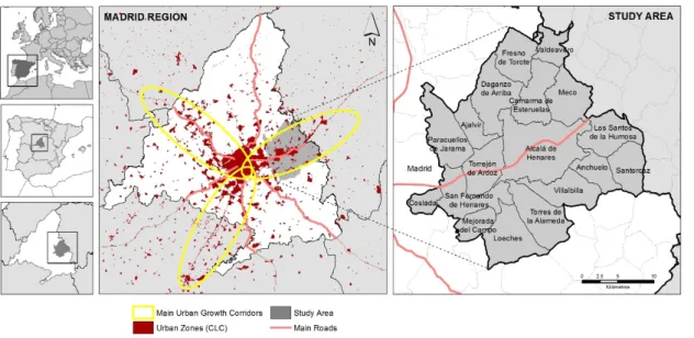
The metropolitan area of Madrid has become one of the most dynamic areas of urban growth in the Iberian Peninsula and Europe [40]. It has three main urban growth corridors, each with their own defining characteristics (Figure1). The study area encompassed 18 municipalities in the Region of Madrid selected from the northeast corridor, known as theCorredor del Henares, which runs from Madrid to Guadalajara (the capital of the neighboring region). This area is home to almost 600,000 inhabitants [41], covers 624 km2, and is strongly influenced by its proximity to the city of Madrid.
In addition, it is a particularly dynamic area in urban and demographic terms, with substantial internal sociodemographic and urban development differences. This complexity is further increased by the lack of regulation aimed at solving territorial problems at the regional level, rendering it an ideal laboratory to test the prototype reported here.
Environments 2018,5, 5 4 of 21
Environments 2018, 5, 5 4 of 21
Figure 1. Urban corridors in the region of Madrid and study area.
The general urban growth trends identified in the main Spanish cities in the period of economic wealth (1997–2007) indicate rapid and chaotic urban development. This coincided with the housing bubble, subsequently followed by a stable period of consolidation [42–44]. Such trends have been witnessed in many other European urban areas in countries, such as Italy, Croatia, and France, mainly associated with their principal cities and coastal zones [45,46].
2.2. Prototype Structure, Platform and Database
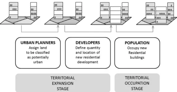
The urban growth process at the regional scale could be theoretically and logically described as a three-stage process involving three types of agent: urban planners, developers, and the population [47]. The first two are responsible for the territorial expansion itself, while the latter represents the occupation of the territory, and all three converge to shape a complex urban system. The urban growth process starts with the identification of new potential urban areas by urban planners in line with national, regional, and local policies. In the second stage, developers choose where to promote new residential developments. Finally, the population selects where to live based on their individual preferences and according to their income possibilities. Although other elements may also be involved in the urban development process (such as infrastructure expansion or political guidelines), these would have been difficult to include in our model, so we decided to limit our agents to these three. Each of them is considered in an independent submodel with different characteristics. The first represents the typical deterministic, top-down process, while the second may be considered a transition between deterministic and stochastic approaches, and the third could be considered the closest representation of an ABM as we understand it (using a bottom-up approach), where complex interactions between agents are represented stochastically. The three of them are coordinated separately before subsequent integration in a final model, where outputs and inputs feed each other continuously. It is worth mentioning that the model is explicitly spatial, so all variables are spatially distributed.
The prototype is intended to be as useful as possible, and therefore it was constructed using an adaptable structure of submodels, each covering a critical variable in the urban growth process. This approach was adopted in response to the low impact that urban growth simulations have had on real-life planning processes, due to their closed architecture and the high amount of data needed to run them, not commonly available in many regions or countries [2].
As presented in Cantergiani et al. [48] the submodels are described below:
The first submodel (urban planner) simulates the urban planner´s decision-making process, which consists of selecting new areas for urban development according to physical restrictions (e.g., protected
Figure 1.Urban corridors in the region of Madrid and study area.
The general urban growth trends identified in the main Spanish cities in the period of economic wealth (1997–2007) indicate rapid and chaotic urban development. This coincided with the housing bubble, subsequently followed by a stable period of consolidation [42–44]. Such trends have been witnessed in many other European urban areas in countries, such as Italy, Croatia, and France, mainly associated with their principal cities and coastal zones [45,46].
2.2. Prototype Structure, Platform and Database
The urban growth process at the regional scale could be theoretically and logically described as a three-stage process involving three types of agent: urban planners, developers, and the population [47].
The first two are responsible for the territorial expansion itself, while the latter represents the occupation of the territory, and all three converge to shape a complex urban system. The urban growth process starts with the identification of new potential urban areas by urban planners in line with national, regional, and local policies. In the second stage, developers choose where to promote new residential developments. Finally, the population selects where to live based on their individual preferences and according to their income possibilities. Although other elements may also be involved in the urban development process (such as infrastructure expansion or political guidelines), these would have been difficult to include in our model, so we decided to limit our agents to these three. Each of them is considered in an independent submodel with different characteristics. The first represents the typical deterministic, top-down process, while the second may be considered a transition between deterministic and stochastic approaches, and the third could be considered the closest representation of an ABM as we understand it (using a bottom-up approach), where complex interactions between agents are represented stochastically. The three of them are coordinated separately before subsequent integration in a final model, where outputs and inputs feed each other continuously. It is worth mentioning that the model is explicitly spatial, so all variables are spatially distributed.
The prototype is intended to be as useful as possible, and therefore it was constructed using an adaptable structure of submodels, each covering a critical variable in the urban growth process.
This approach was adopted in response to the low impact that urban growth simulations have had on real-life planning processes, due to their closed architecture and the high amount of data needed to run them, not commonly available in many regions or countries [2].
As presented in Cantergiani et al. [48] the submodels are described below:
The first submodel (urban planner) simulates the urban planner´s decision-making process, which consists of selecting new areas for urban development according to physical restrictions (e.g., protected
areas, high slopes, or proximity to water bodies), distance to elements of interest (e.g., roads or consolidated urban areas), and the amount of growth required to meet existing demand. These criteria are set as parameters and can be modified at initialization to generate different scenarios.
The second submodel (developer) focuses on the developer’s decision-making process regarding new residential developments. As part of their behavior, developers must decide where to build new housing, how many new developments must be built, their capacity, and their target economic group.
This process takes into account the legal status of the territory (defined by urban planners in the first submodel), as well as the areas that will optimize their profits.
The third submodel (population) simulates the process of residential location choice and occupation by the population. In this case, different agents look for the best place to move according to their purchasing power and location preferences, which may include distance to the public transport network, education facilities, and other factors.
The flowchart in Figure2shows how the submodels are integrated and where the result of each submodel feeds into the next in a chain-like process.
Environments 2018, 5, 5 5 of 21
areas, high slopes, or proximity to water bodies), distance to elements of interest (e.g., roads or consolidated urban areas), and the amount of growth required to meet existing demand. These criteria are set as parameters and can be modified at initialization to generate different scenarios.
The second submodel (developer) focuses on the developer’s decision-making process regarding new residential developments. As part of their behavior, developers must decide where to build new housing, how many new developments must be built, their capacity, and their target economic group. This process takes into account the legal status of the territory (defined by urban planners in the first submodel), as well as the areas that will optimize their profits.
The third submodel (population) simulates the process of residential location choice and occupation by the population. In this case, different agents look for the best place to move according to their purchasing power and location preferences, which may include distance to the public transport network, education facilities, and other factors.
The flowchart in Figure 2 shows how the submodels are integrated and where the result of each submodel feeds into the next in a chain-like process.
Figure 2. Integrated decision model to simulate urban growth.
The conceptual model considers two components for the three agents: territorial availability (TA) and spatial interest criteria (SIC). The first (TA) indicates potential areas taking into account spatial restrictions. For urban planners, it considers the limits imposed by legal regulations (e.g., master plans, law on protected areas) and physical urban development restrictions (e.g., along rivers, steep slopes) to spatially delineate potential areas for development. For developers, TA restricts the area to those classified as potentially urban. The second component (SIC) represents attractiveness, which indicates the preferences of each agent regarding the distance to given spatial elements. For urban planners, these include roads, public facilities, hazardous areas, agricultural productivity, and existing urban fabric, while for developers they include roads, public transport stops, existing urban fabric, and status of the existing residential stock. Due to the flexibility of each submodel of the prototype, several variables can be selected to represent these components and run the model [47], although here we only report those tested in the study area.
The platform used to develop the prototype was NetLogo v.5.3.1 (Center for Connected Learning and Computer-Based Modeling, Northwestern University, Evanston-IL, IL, USA) [49], which met the technical requirements and presents many advantages. To name a few, it has an intuitive and simple interface, it is widely used for similar applications, it is user-friendly, and it is open source. Moreover, it enables simple connection with geographical databases through a Geographic Information System (GIS) extension, fundamental for spatial analysis. For instance, this
Figure 2.Integrated decision model to simulate urban growth.
The conceptual model considers two components for the three agents: territorial availability (TA) and spatial interest criteria (SIC). The first (TA) indicates potential areas taking into account spatial restrictions. For urban planners, it considers the limits imposed by legal regulations (e.g., master plans, law on protected areas) and physical urban development restrictions (e.g., along rivers, steep slopes) to spatially delineate potential areas for development. For developers, TA restricts the area to those classified as potentially urban. The second component (SIC) represents attractiveness, which indicates the preferences of each agent regarding the distance to given spatial elements. For urban planners, these include roads, public facilities, hazardous areas, agricultural productivity, and existing urban fabric, while for developers they include roads, public transport stops, existing urban fabric, and status of the existing residential stock. Due to the flexibility of each submodel of the prototype, several variables can be selected to represent these components and run the model [47], although here we only report those tested in the study area.
The platform used to develop the prototype was NetLogo v.5.3.1 (Center for Connected Learning and Computer-Based Modeling, Northwestern University, Evanston-IL, IL, USA) [49], which met the technical requirements and presents many advantages. To name a few, it has an intuitive and simple interface, it is widely used for similar applications, it is user-friendly, and it is open source.
Moreover, it enables simple connection with geographical databases through a Geographic Information System (GIS) extension, fundamental for spatial analysis. For instance, this connection facilitates the
Environments 2018,5, 5 6 of 21
flexibility required for adaptation to other study areas, with different input data in terms of extension or resolution.
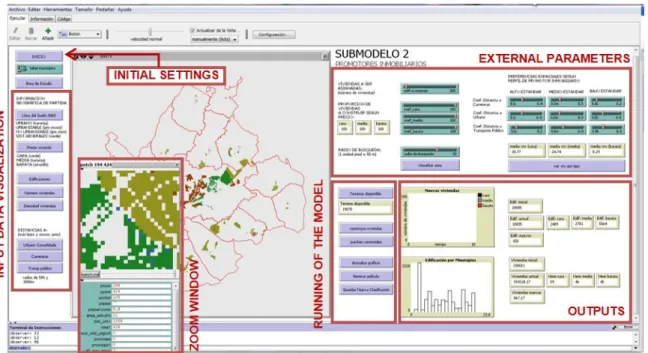
The submodel interface consists of three sections: (i) an input box where geographical information is called up and spatially represented in a visualization panel; (ii) an area where the user sets the initial parameters that will define the scenarios to simulate; and finally (iii) a third area where the results are represented in the form of graphs, spatial distribution, and an external matrix containing statistical references (Figure3).
Environments 2018, 5, 5 6 of 21
connection facilitates the flexibility required for adaptation to other study areas, with different input data in terms of extension or resolution.
The submodel interface consists of three sections: (i) an input box where geographical information is called up and spatially represented in a visualization panel; (ii) an area where the user sets the initial parameters that will define the scenarios to simulate; and finally (iii) a third area where the results are represented in the form of graphs, spatial distribution, and an external matrix containing statistical references (Figure 3).
Figure 3. Distribution of the functional blocks in the interface (common for all submodels).
All submodels have a similar interface, differing only in the number and kind of external parameters to be set, and obviously in the expected outputs. Since a set of parameters can be freely modeled, users can adapt the model to their specific context and generate different future urban growth scenarios.
Bearing in mind the regional scale and main drivers of urban growth in the context cited and other similar contexts, a considerable effort was made to compile the most appropriate alphanumerical and geographical information, always considering the territorial component.
Although they might form part of the process, statistical components were only incorporated into the model when they could be spatially represented (such as price and income distribution). Other variables, such as traffic flows, global climate change, mobility, and time variation, were not included at this stage for the abovementioned reasons, although we recognize they must play a partial role in the evolution of the phenomenon studied.
The input data used to implement the submodels were selected to reflect the drivers of urban growth, empirical knowledge of urban growth trends in the study area [47,48,50,51], and the most commonly used variables in other studies [8,33]. These latter included the municipal boundaries (surface), zoning status (surface), and housing distribution (pixel) used by agents to assess specific environments and conditions, as well as the other spatial information indicated in Table 1 below.
These were represented by pixels measuring 50 × 50 m. Once data had been collected, they were transformed into determinants for subsequent use in the model.
Figure 3.Distribution of the functional blocks in the interface (common for all submodels).
All submodels have a similar interface, differing only in the number and kind of external parameters to be set, and obviously in the expected outputs. Since a set of parameters can be freely modeled, users can adapt the model to their specific context and generate different future urban growth scenarios.
Bearing in mind the regional scale and main drivers of urban growth in the context cited and other similar contexts, a considerable effort was made to compile the most appropriate alphanumerical and geographical information, always considering the territorial component. Although they might form part of the process, statistical components were only incorporated into the model when they could be spatially represented (such as price and income distribution). Other variables, such as traffic flows, global climate change, mobility, and time variation, were not included at this stage for the abovementioned reasons, although we recognize they must play a partial role in the evolution of the phenomenon studied.
The input data used to implement the submodels were selected to reflect the drivers of urban growth, empirical knowledge of urban growth trends in the study area [47,48,50,51], and the most commonly used variables in other studies [8,33]. These latter included the municipal boundaries (surface), zoning status (surface), and housing distribution (pixel) used by agents to assess specific environments and conditions, as well as the other spatial information indicated in Table1below.
These were represented by pixels measuring 50×50 m. Once data had been collected, they were transformed into determinants for subsequent use in the model.
Table 1.Description of determinants, based on input data, incorporated into the prototype.
Data Layer Scale Origin Determinant and Description
Census zones and associated
statistical data 1:1000 INE (2001)
Distance to consolidated urban zones Contributes to determination of
agents’ preferences
Zoning status 1:50,000
Department of Environment, Housing and Land Use Planning, Region of Madrid
(2006)
Land classification (reclassified as urban, non-building, and potentially urban)
Functions as the legal constraint on agents’ actions Natural Protected Zones
(Spanish initials: ENP) 1:50,000
Environment Database of Spanish Ministry of the
Environment (2012)
Restricted areas (sum of individual restrictions spatially distributed) These act as a mask under which agents
cannot intercede Buffer along main water bodies 1:25,000 BCN 25/CNIG, IGN (2008)
Slope (origin: Digital Terrain Model) 1:50,000 BCN 25/CNIG, IGN (2012)
Land use and land cover 1:100,000 CORINE Land Cover Project of IGN (2000–2005)
Agricultural productivity generated from reclassification of the land use database Agents state their preferences according to
the high, medium, or low level of productivity Urban facilities (health and
education, public transport, locally unwanted land uses)
1:25,000
NomeCalles Database of Statistical Institute of Region
of Madrid (2005)
Distance to each type of facility This may indicate a higher or lower level
of interest Cadastral data containing
information at parcel level (code, municipality, use, year of construction, area, centroid, etc.)
1:1000
General Directorate for Land Register, Ministry of Finance and Public Administration
(2006)
Aggregated data by pixel represent the initial residential building distribution
Agents behave according to the existing buildings
Network of national and
regional roads 1:25,000 BCN 25/CNIG, IGN (2008)
Accessibility calculated as distance to the road network
This may indicate a higher or lower level of interest
INE: National Statistics Institute; BCN: National Cartographic Database; CNIG: National Center for Geographical Information; IGN: National Geographic Institute; ENP: Protected Natural Spaces.
3. Implementation of the Territorial Expansion Simulation
3.1. Urban Planner Submodel
The urban planner submodel simulates regional urban growth and represents the most general scale of the three submodels, indicating areas where it is legally permissible to construct new residential buildings. This submodel presents a simple and deterministic structure, since the behavior of urban planners generally reflects a top-down approach whereby decisions are made within a general plan by an institutional agent rather than by individuals (or by an individual representing an institution).
Nonetheless, the allocation model was developed in NetLogo in order to facilitate integration into future submodels that might simulate agents’ behavior using the bottom-up approach.
The expected result is useful for any urban planner, and represents a laboratory that allows the selection of new areas for reclassification as potentially urban (Figure4), generated from their decision regarding the most suitable areas according to criteria that may differ depending on the agent’s profile.
Rather than testing the model with different types of urban planner, we only considered one type presenting different profiles that in turn could generate numerous scenarios.
Environments 2018,5, 5 8 of 21
Environments 2018, 5, 5 8 of 21
Figure 4. Conceptual decision structure of the urban planner submodel.
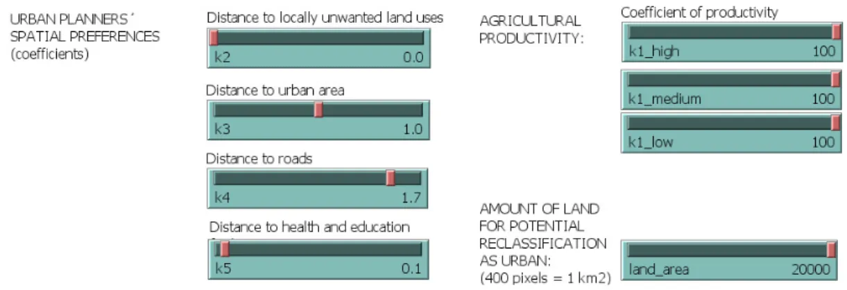
Besides defining the amount of land for potential reclassification as urban, the interface allows the user to set initial conditions that characterize each profile (Figure 5). Hence, the interface settings allow the user to establish weights for variables such as distance to urban areas, locally unwanted land uses (e.g., hazardous waste dumps, prisons, and trash disposal plants), road infrastructures, and health/education services, and to define priority areas for potential reclassification as urban according to their agricultural productivity.
Figure 5. Variables that can be set when initializing the model to define different urban planner profiles.
The agent must convert the amount of land specified by the user in the interface, and the simulation outcomes should show where these changes will take place. The model mechanism works as follows: from among the non-restricted surface areas—limited according to user selection from among the three available options—urban planners first analyze those areas with the highest values of interest. These values are graduated using the average of the weights indicated on the sliders at the interface for each pixel (Figure 5). Then, the last coefficient (agricultural productivity) is set, and the model assumes that the proposed percentage is homogeneously distributed spatially and randomly throughout each area according to its agricultural productivity, defined as high (forest and natural areas), medium (agricultural areas), or low (all other categories) based on a reclassification of
Figure 4.Conceptual decision structure of the urban planner submodel.
Besides defining the amount of land for potential reclassification as urban, the interface allows the user to set initial conditions that characterize each profile (Figure5). Hence, the interface settings allow the user to establish weights for variables such as distance to urban areas, locally unwanted land uses (e.g., hazardous waste dumps, prisons, and trash disposal plants), road infrastructures, and health/education services, and to define priority areas for potential reclassification as urban according to their agricultural productivity.
Environments 2018, 5, 5 8 of 21
Figure 4. Conceptual decision structure of the urban planner submodel.
Besides defining the amount of land for potential reclassification as urban, the interface allows the user to set initial conditions that characterize each profile (Figure 5). Hence, the interface settings allow the user to establish weights for variables such as distance to urban areas, locally unwanted land uses (e.g., hazardous waste dumps, prisons, and trash disposal plants), road infrastructures, and health/education services, and to define priority areas for potential reclassification as urban according to their agricultural productivity.
Figure 5. Variables that can be set when initializing the model to define different urban planner profiles.
The agent must convert the amount of land specified by the user in the interface, and the simulation outcomes should show where these changes will take place. The model mechanism works as follows: from among the non-restricted surface areas—limited according to user selection from among the three available options—urban planners first analyze those areas with the highest values of interest. These values are graduated using the average of the weights indicated on the sliders at the interface for each pixel (Figure 5). Then, the last coefficient (agricultural productivity) is set, and the model assumes that the proposed percentage is homogeneously distributed spatially and randomly throughout each area according to its agricultural productivity, defined as high (forest and natural areas), medium (agricultural areas), or low (all other categories) based on a reclassification of
Figure 5.Variables that can be set when initializing the model to define different urban planner profiles.
The agent must convert the amount of land specified by the user in the interface, and the simulation outcomes should show where these changes will take place. The model mechanism works as follows: from among the non-restricted surface areas—limited according to user selection from among the three available options—urban planners first analyze those areas with the highest values of interest. These values are graduated using the average of the weights indicated on the sliders at the interface for each pixel (Figure5). Then, the last coefficient (agricultural productivity) is set, and the model assumes that the proposed percentage is homogeneously distributed spatially and randomly throughout each area according to its agricultural productivity, defined as high (forest and natural areas), medium (agricultural areas), or low (all other categories) based on a reclassification of the
CORINE Land Cover land use categories considered artificial [52]. The final selection is then taken as the best option.
Having described and implemented the conceptual model in NetLogo, the simulation experiments conducted to test the prototype are reported below. Several authors have suggested that the validation process should consist of different components: verification, validation, and a sensitivity analysis [12,53–58]. However, since this paper presents a prototype of an ABM, it focuses less on predicting the future and more on understanding and exploring the behavior of the urban system and reproducing specific scenarios. Consequently, only verification of correct model construction and validation by comparing the results with real data will be discussed further. Verification (also known as internal validation) refers to the correctness of the internal structure, ensuring that the model has been developed in a formally correct manner (e.g., system diagrams, units of measurement, and equations) in accordance with a specified methodology [58]. This implies corroborating that the implemented model conforms to the specifications by running it after changing some initial parameters, as done by other modelers [33]. Statistical validation, or just validation, refers to determining if the model is correct by checking whether it achieves the expected level of accuracy in its predictions. This involves analyzing whether the structure of the model is appropriate for its intended purpose from a conceptual and operational point of view by comparing results to real data.
The goal of these procedures was twofold: on the one hand, to confirm that the results of specific scenarios could help determine whether the model had been correctly constructed, and on the other, to confirm that the model has the capacity to generate the expected simulation, given the scale, available data, and initial set of conditions.
For verification, three different contexts were set for each model by varying some of the initial parameters (e.g., adopting a sustainable, economically conservative, or speculative approach), so that they were sufficiently diverse to generate different outputs. It is important to note that throughout this paper, the term “scenarios” is used to refer to different future contexts, rather than according to the definition of scenario in the strict sense of the term. Moreover, all of the prototype submodels represent tools in the form of open possibilities that can reproduce different urban development scenarios (as reported here) and generate a sequence of products that could be used for a validation process such as a sensitivity analysis, employed by many scientists for this purpose [16,18,36]. We propose to conduct such an analysis on the final model once all three submodels have been integrated.
Hence, although very different results could arise from minor changes in these initial conditions, the usefulness of the simulations resides in the fact that they were not aimed at identifying or analyzing specific urban growth shapes or statistics for theCorredor del Henares, but at determining whether the model was correctly constructed. If this latter were to be demonstrated, it would support the notion that ABM constitute a powerful tool for use in real situations and would confirm that the prototype achieves the proposed goal. The flexibility and high number of setting options increase the possibility of employing this tool in different contexts and using real data on other areas.
For the validation process, we compared the results of the different simulations (of the two submodels once integrated) with the corresponding urban land data available for the study area, and obtained the percentage of coincidence.
With these goals in mind, we simulated the expansion of potential development areas using three different urban planner profiles defined by the tendency to employ: (i) a sustainable approach, (ii) an economically conservative approach (typical behavior in a crisis situation), or (iii) a speculative approach (corresponding to a business-as-usual scenario), in accordance with the storyline and scenarios described in Plata Rocha et al. [50]. In order to run the three simulations, the same initial conditions were used, but different parameters were set to characterize each profile (Table2), based on the work cited. As expected, the simulations yielded some notable differences for the three urban planner profiles, all of them with growth concentrated close to the most dynamic existing urban areas, but distributed differently throughout the territory. Other future contexts could be easily defined by changing values for each parameter.
Environments 2018,5, 5 10 of 21
Table 2.Initial conditions for three different urban planner profiles.
Variable/Urban Planner Profile Reference Sustainable Conservative Speculative
Distance to locally unwanted land uses * 0.0 to 2.0 1.0 0.0 0.0
Distance to urban areas * 0.0 to 2.0 1.0 2.0 0.5
Distance to roads * 0.0 to 2.0 2.0 1.5 0.5
Distance to health and education facilities * 0.0 to 2.0 2.0 1.0 0.0
Agricultural productivity:
Conversion to potential building land in zones
with high agricultural productivity (%) 0 to 100 0 5% 20%
Conversion to potential building land in zones
with medium agriculture productivity level (%) 0 to 100 10% 20% 40%
Conversion to potential building land in zones
with low agricultural productivity (%) 0 to 100 90% 75% 40%
* Zero indicates that this factor is not relevant, while two indicates maximum relevance. Intermediate values show proximity to minimum or maximum influence.
Therefore, the simulation results are acceptable since they are spatially and conceptually coherent.
An aggregated visualization of real data on the evolution of past and recent urban plans (the municipalities in the study area have relatively old plans and many updates are under discussion) and simulation with a five-year horizon for the three planner profiles (Figure6) indicate alternative distributions that could be used as a reference for urban planning decision-making.
Environments 2018, 5, 5 10 of 21
Table 2. Initial conditions for three different urban planner profiles.
Variable/Urban Planner Profile Reference Sustainable Conservative Speculative Distance to locally unwanted land uses * 0.0 to 2.0 1.0 0.0 0.0
Distance to urban areas * 0.0 to 2.0 1.0 2.0 0.5
Distance to roads * 0.0 to 2.0 2.0 1.5 0.5
Distance to health and education facilities * 0.0 to 2.0 2.0 1.0 0.0 Agricultural productivity:
Conversion to potential building land in
zones with high agricultural productivity (%) 0 to 100 0 5% 20%
Conversion to potential building land in zones with medium agriculture productivity level (%)
0 to 100 10% 20% 40%
Conversion to potential building land in
zones with low agricultural productivity (%) 0 to 100 90% 75% 40%
* Zero indicates that this factor is not relevant, while two indicates maximum relevance. Intermediate values show proximity to minimum or maximum influence.
Therefore, the simulation results are acceptable since they are spatially and conceptually coherent. An aggregated visualization of real data on the evolution of past and recent urban plans (the municipalities in the study area have relatively old plans and many updates are under discussion) and simulation with a five-year horizon for the three planner profiles (Figure 6) indicate alternative distributions that could be used as a reference for urban planning decision-making.
Figure 6. Comparison of simulation results (five years) and real data on past urban plans for the three planner profiles: (a) sustainable, (b) conservative, (c) speculative.
Figure 6.Comparison of simulation results (five years) and real data on past urban plans for the three planner profiles: (a) sustainable, (b) conservative, (c) speculative.
3.2. Developer Submodel
The developer submodel considers a bottom-up rather than a top-down approach [27], assuming a more spatially-restricted knowledge of the territory (in the urban planner submodel, agents are assumed to be familiar with the entire territory in order to make a decision). Simulation of their behavior is expected to yield a new distribution of low, medium, and high standard residential buildings.
In the first instance, the only restrictions (TA) considered referred to regulations; thus, only already- designated areas were candidates for new residential development. As regards attractiveness (SIC), the preferred distance to elements of spatial interest was defined according to the standard of the building for which expansion was to be simulated. In this model, land value and neighborhood characteristics were the two main elements that strongly affected the decision to assign a new area for development (Figure7).
3.2. Developer Submodel
The developer submodel considers a bottom-up rather than a top-down approach [27], assuming a more spatially-restricted knowledge of the territory (in the urban planner submodel, agents are assumed to be familiar with the entire territory in order to make a decision). Simulation of their behavior is expected to yield a new distribution of low, medium, and high standard residential buildings.
In the first instance, the only restrictions (TA) considered referred to regulations; thus, only already-designated areas were candidates for new residential development. As regards attractiveness (SIC), the preferred distance to elements of spatial interest was defined according to the standard of the building for which expansion was to be simulated. In this model, land value and neighborhood characteristics were the two main elements that strongly affected the decision to assign a new area for development (Figure 7).
Figure 7. Conceptual decision structure of the developer submodel. #: number.
As in the previous case, agents in this submodel present a unique type of behavior regarding the variables considered, although users may change some of the parameters depending on whether they aim to simulate the construction of high-, medium-, or low-standard housing. In addition, the interface again allows the user to establish the initial conditions by changing parameters such as the quantification of new buildings, specification of respective percentage of each type, and calibration of available coefficients for each standard (distance to roads, urban areas, and public transport). The user can also define the maximum search area that developers should take into account, considering the elements necessary to identify a suitable location (where no ideal location is identified within the area defined, the model allows the user to redefine the search area). The combination of these parameters defines the future scenario.
The decision flow chart (Figure 8) leads to the final location where new housing should be built.
Unlike the urban planner submodel, the developer submodel starts with the selection of the typology of building proposed, i.e., whether the agent will seek free land to build high, medium, or low standard housing. This information is vital to confirm the area of interest, which is different for each case, and later it will also be useful to define the number of dwellings assigned to each new building typology. This choice must respect the maximum allowed for each typology. In the next step, the model focuses on a random point that must obey the restrictions and analyzes the neighborhood, considering an extension which is also indicated in the interface by the user. The
Figure 7.Conceptual decision structure of the developer submodel. #: number.
As in the previous case, agents in this submodel present a unique type of behavior regarding the variables considered, although users may change some of the parameters depending on whether they aim to simulate the construction of high-, medium-, or low-standard housing. In addition, the interface again allows the user to establish the initial conditions by changing parameters such as the quantification of new buildings, specification of respective percentage of each type, and calibration of available coefficients for each standard (distance to roads, urban areas, and public transport). The user can also define the maximum search area that developers should take into account, considering the elements necessary to identify a suitable location (where no ideal location is identified within the area defined, the model allows the user to redefine the search area). The combination of these parameters defines the future scenario.
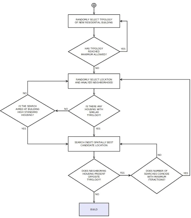
The decision flow chart (Figure8) leads to the final location where new housing should be built.
Unlike the urban planner submodel, the developer submodel starts with the selection of the typology of building proposed, i.e., whether the agent will seek free land to build high, medium, or low standard housing. This information is vital to confirm the area of interest, which is different for each case, and later it will also be useful to define the number of dwellings assigned to each new building typology. This choice must respect the maximum allowed for each typology. In the next step, the model focuses on a random point that must obey the restrictions and analyzes the neighborhood,
Environments 2018,5, 5 12 of 21
considering an extension which is also indicated in the interface by the user. The preference criteria include the degree of similarity with nearby buildings (attraction for similar, or in some cases, rejection for different) and the spatial interest defined as in the previous submodel. Whenever there is an option that complies with these criteria, and the maximum number of runs has not yet been reached, the new building is assigned to the corresponding pixel. The number of dwellings assigned will depend on building typology, going from high density (low standard) to low density (high standard).
Environments 2018, 5, 5 12 of 21
preference criteria include the degree of similarity with nearby buildings (attraction for similar, or in some cases, rejection for different) and the spatial interest defined as in the previous submodel.
Whenever there is an option that complies with these criteria, and the maximum number of runs has not yet been reached, the new building is assigned to the corresponding pixel. The number of dwellings assigned will depend on building typology, going from high density (low standard) to low density (high standard).
Figure 8. Developer’s decision flow chart.
As in the previous case, in order to confirm prototype flexibility and correct construction, scenarios were defined according to the external environment rather than the agent’s profile (as in submodel 1). In this case, two parameters could be modified: the residential growth predicted for each housing standard and the maximum search area. In order to test the model, different settings were defined for these parameters in order to simulate the real estate market under three different situations: (i) sustainable (environmental protection approach), (ii) crisis (conservative approach) and (iii) speculative (business as usual). Each scenario reflects different building dynamics, housing
Figure 8.Developer’s decision flow chart.
As in the previous case, in order to confirm prototype flexibility and correct construction, scenarios were defined according to the external environment rather than the agent’s profile (as in submodel 1).
In this case, two parameters could be modified: the residential growth predicted for each housing standard and the maximum search area. In order to test the model, different settings were defined for these parameters in order to simulate the real estate market under three different situations:
(i) sustainable (environmental protection approach), (ii) crisis (conservative approach) and (iii)
speculative (business as usual). Each scenario reflects different building dynamics, housing typology distribution balance, and urban growth shape, all defined by adjusting the values for the initial submodel conditions (Table3).
Table 3. Initial settings and description of submodel spatial results from simulation of the three developer scenarios.
Scenario Initial Settings Description of Results
Characteristics that
represent the scenario Building dynamics Housing typology
distribution balance Urban growth shape
Equivalent parameter in the submodel interface
Number of residential buildings (100–3000)
% of growth for high, medium, or low standard buildings
(0–100%)
Compact or disseminated represented by the search area size (50–1500 m)
Scenario 1: Sustainable High (3500 new buildings)
Balanced (high for all,
mean: 70%) Narrow (500 m)
Group of buildings in a compact shape, usually
connected to existing buildings
Scenario 2: Crisis Low (500 new buildings)
Unbalanced (low for
all, mean: 30%) Narrow (500 m)
Few buildings, distributed evenly, most of them
low standard Scenario 3: Speculative High (3500
new buildings)
Balanced (high for all,
mean: 70%) Wide (1500 m) New buildings dispersed throughout the territory
The last column in Table3presents a short description of the results, indicating satisfactory agreement between the proposal and the expected and simulated results, mainly considering the spatial response for the three situations (Figure9). Furthermore, the final distribution shows the actual and projected housing together, indicating the lack of development in restricted areas (non-building areas or roads, for example). The spatial results for the developed area were generated from pixel distribution over the surface designated for that purpose (urban and developable land). We did not consider illegal settlement dynamics at this stage of the model.
Environments 2018, 5, 5 13 of 21
typology distribution balance, and urban growth shape, all defined by adjusting the values for the initial submodel conditions (Table 3).
Table 3. Initial settings and description of submodel spatial results from simulation of the three developer scenarios.
Scenario Initial Settings Description of Results
Characteristics that represent the scenario
Building dynamics
Housing typology
distribution balance Urban growth shape
Equivalent parameter in the submodel interface
Number of residential buildings (100–3000)
% of growth for high, medium, or low standard buildings
(0–100%)
Compact or disseminated represented by the search area size (50–
1500 m)
Scenario 1: Sustainable
High (3500 new buildings)
Balanced (high for
all, mean: 70%) Narrow (500 m)
Group of buildings in a compact shape, usually connected to existing
buildings
Scenario 2: Crisis Low (500 new buildings)
Unbalanced (low for
all, mean: 30%) Narrow (500 m)
Few buildings, distributed evenly,
most of them low standard Scenario 3: Speculative
High (3500 new buildings)
Balanced (high for
all, mean: 70%) Wide (1500 m)
New buildings dispersed throughout
the territory
The last column in Table 3 presents a short description of the results, indicating satisfactory agreement between the proposal and the expected and simulated results, mainly considering the spatial response for the three situations (Figure 9). Furthermore, the final distribution shows the actual and projected housing together, indicating the lack of development in restricted areas (non- building areas or roads, for example). The spatial results for the developed area were generated from pixel distribution over the surface designated for that purpose (urban and developable land). We did not consider illegal settlement dynamics at this stage of the model.
Figure 9.Cont.
Environments 2018,5, 5 14 of 21
Environments 2018, 5, 5 14 of 21
Figure 9. Spatial results for the three simulation scenarios: (a) sustainable, (b) crisis, and (c) speculative.
3.3. Integration of the Urban Planner and Developer Submodels
Although we only integrated two of three prototype submodels, this still presented a challenge due to the problem of how to combine two different submodels in one, which must also be clear and robust. Below, we describe how this difficulty was solved and the two submodels combined to represent the territorial expansion process:
• The submodels were combined through continuous feedback of inputs and outputs. Thus, the developer submodel uses the output of the urban planner submodel (land classification) as one of the inputs; hence, depending on the established criteria, an updated layer is periodically obtained showing areas classified as potential building land. As developers behave according to these legal restrictions, the results of the independent submodels and integrated model should differ.
• Temporal resolution also presents a challenge because the two submodels use different time intervals to reflect the fact that developers build housing in a shorter period of time than urban planners take to develop new planning proposals. By law in Spain, urban plans must be revised at least every ten years with some periodical, partial reviews; thus, five years was the interval considered for the urban planner submodel, although it could easily be modified according to where the prototype is being employed. For the developer submodel, we considered an interval of one year to reflect the time taken to construct new residential housing, although we are aware that this is often a continuous process.
• Successful integration of the two submodels depended not only on which inputs/outputs were considered, but also on when and how they were interchanged, since the submodels employ different time intervals. The rate is determined by compliance with criteria that interrupt the running of one submodel to start that of the other. In order to obtain the first results, to skip from the developer to the urban planner submodel, either (i) the free area suitable for development should not exceed a defined percentage of the total, or (ii) one of the submodels should reach a given number of runs (Figure 10).
In summary, the model starts with a territory classified into urban, potentially urban, and other, and also with a fixed distribution of buildings. The prototype internally calculates the percentage of potentially urban areas occupied by residential buildings and the number of runs for each (starting from zero). If the result exceeds the amount defined by the user (meaning that new areas are in demand), then the urban planner submodel is launched. Otherwise, the developer submodel is run continuously until that percentage is reached. Both submodels run in accordance with the independent procedures described previously. In this case, the NetLogo platform was selected in Figure 9.Spatial results for the three simulation scenarios: (a) sustainable, (b) crisis, and (c) speculative.
3.3. Integration of the Urban Planner and Developer Submodels
Although we only integrated two of three prototype submodels, this still presented a challenge due to the problem of how to combine two different submodels in one, which must also be clear and robust. Below, we describe how this difficulty was solved and the two submodels combined to represent the territorial expansion process:
• The submodels were combined through continuous feedback of inputs and outputs. Thus, the developer submodel uses the output of the urban planner submodel (land classification) as one of the inputs; hence, depending on the established criteria, an updated layer is periodically obtained showing areas classified as potential building land. As developers behave according to these legal restrictions, the results of the independent submodels and integrated model should differ.
• Temporal resolution also presents a challenge because the two submodels use different time intervals to reflect the fact that developers build housing in a shorter period of time than urban planners take to develop new planning proposals. By law in Spain, urban plans must be revised at least every ten years with some periodical, partial reviews; thus, five years was the interval considered for the urban planner submodel, although it could easily be modified according to where the prototype is being employed. For the developer submodel, we considered an interval of one year to reflect the time taken to construct new residential housing, although we are aware that this is often a continuous process.
• Successful integration of the two submodels depended not only on which inputs/outputs were considered, but also on when and how they were interchanged, since the submodels employ different time intervals. The rate is determined by compliance with criteria that interrupt the running of one submodel to start that of the other. In order to obtain the first results, to skip from the developer to the urban planner submodel, either (i) the free area suitable for development should not exceed a defined percentage of the total, or (ii) one of the submodels should reach a given number of runs (Figure10).
In summary, the model starts with a territory classified into urban, potentially urban, and other, and also with a fixed distribution of buildings. The prototype internally calculates the percentage of potentially urban areas occupied by residential buildings and the number of runs for each (starting from zero). If the result exceeds the amount defined by the user (meaning that new areas are in demand), then the urban planner submodel is launched. Otherwise, the developer submodel is run continuously until that percentage is reached. Both submodels run in accordance with the independent procedures described previously. In this case, the NetLogo platform was selected in order to better
integrate both of these with each other and with the third population submodel in an ABM context, since other techniques such as CA or multi-criteria models might not be able to solve integration.
order to better integrate both of these with each other and with the third population submodel in an ABM context, since other techniques such as CA or multi-criteria models might not be able to solve integration.
(a) (b)
Figure 10. Sequential flow considering compliance or not with the criteria in order to skip from one model to the other: (a) Continuous cycle, (b) Cycle when “skip” conditions are met. SM1: submodel 1—urban planners; SM2: submodel 2—developers.
In order to conduct initial integration of the submodels, we considered a fixed sustainable scenario for both. In the first instance, this should represent the ideal approach to urban development, taking into consideration legal and strategic factors. Although this variable would depend entirely on the user’s interests, for this simulation experiment we set the urban planner submodel to run once for each three runs of the developer submodel, with the latter running at one-year intervals. As expected, the results of this integrated simulation indicated urban growth along roads and around existing developments: potential urban land expansion occurred close to residential buildings in the smaller municipalities, and mainly in the central ones (Figure 11).
Figure 11. Interface of the model that integrates the urban planner and developer submodels and results shown in a Geographic Information System (GIS).
Figure 10.Sequential flow considering compliance or not with the criteria in order to skip from one model to the other: (a) Continuous cycle, (b) Cycle when “skip” conditions are met. SM1: submodel 1—urban planners; SM2: submodel 2—developers.
In order to conduct initial integration of the submodels, we considered a fixed sustainable scenario for both. In the first instance, this should represent the ideal approach to urban development, taking into consideration legal and strategic factors. Although this variable would depend entirely on the user’s interests, for this simulation experiment we set the urban planner submodel to run once for each three runs of the developer submodel, with the latter running at one-year intervals. As expected, the results of this integrated simulation indicated urban growth along roads and around existing developments: potential urban land expansion occurred close to residential buildings in the smaller municipalities, and mainly in the central ones (Figure11).
Environments 2018, 5, 5 15 of 21
order to better integrate both of these with each other and with the third population submodel in an ABM context, since other techniques such as CA or multi-criteria models might not be able to solve integration.
(a) (b)
Figure 10. Sequential flow considering compliance or not with the criteria in order to skip from one model to the other: (a) Continuous cycle, (b) Cycle when “skip” conditions are met. SM1: submodel 1—urban planners; SM2: submodel 2—developers.
In order to conduct initial integration of the submodels, we considered a fixed sustainable scenario for both. In the first instance, this should represent the ideal approach to urban development, taking into consideration legal and strategic factors. Although this variable would depend entirely on the user’s interests, for this simulation experiment we set the urban planner submodel to run once for each three runs of the developer submodel, with the latter running at one-year intervals. As expected, the results of this integrated simulation indicated urban growth along roads and around existing developments: potential urban land expansion occurred close to residential buildings in the smaller municipalities, and mainly in the central ones (Figure 11).
Figure 11. Interface of the model that integrates the urban planner and developer submodels and results shown in a Geographic Information System (GIS).
Figure 11. Interface of the model that integrates the urban planner and developer submodels and results shown in a Geographic Information System (GIS).