An Introduction to Acceptance Sampling and SPC with R (John Lawson) (z-lib.org)

(1)

(2)

An Introduction to Acceptance Sampling

and SPC with R

(3)

(4)

An Introduction to Acceptance Sampling

and SPC with R

John Lawson

(5)

by CRC Press

6000 Broken Sound Parkway NW, Suite 300, Boca Raton, FL 33487-2742 and by CRC Press

2 Park Square, Milton Park, Abingdon, Oxon, OX14 4RN

CRC Press is an imprint of Taylor & Francis Group, LLC

The right of John Lawson to be identified as author of this work has been asserted by him in accor- dance with sections 77 and 78 of the Copyright, Designs and Patents Act 1988.

Reasonable efforts have been made to publish reliable data and information, but the author and pub- lisher cannot assume responsibility for the validity of all materials or the consequences of their use.

The authors and publishers have attempted to trace the copyright holders of all material reproduced in this publication and apologize to copyright holders if permission to publish in this form has not been obtained. If any copyright material has not been acknowledged please write and let us know so we may rectify in any future reprint.

Except as permitted under U.S. Copyright Law, no part of this book may be reprinted, reproduced, transmitted, or utilized in any form by any electronic, mechanical, or other means, now known or hereafter invented, including photocopying, microfilming, and recording, or in any information stor- age or retrieval system, without written permission from the publishers.

For permission to photocopy or use material electronically from this work, access www.copyright.com or contact the Copyright Clearance Center, Inc. (CCC), 222 Rosewood Drive, Danvers, MA 01923, 978- 750-8400. For works that are not available on CCC please contact [email protected] Trademark notice: Product or corporate names may be trademarks or registered trademarks, and are used only for identification and explanation without intent to infringe.

ISBN: 9780367569952 (hbk) ISBN: 9780367555764 (pbk) ISBN: 9781003100270 (ebk) Typeset in Computer Modern font by KnowledgeWorks Global Ltd.

Access the Support Material: https://www.routledge.com/9780367555764

(6)

Preface ix

List of Figures xiii

List of Tables xvii

1 Introduction and Historical Background 1

1.1 Origins of Statistical Quality Control . . . 1

1.2 Expansion and Development of Statistical Quality Control during WW II . . . 3

1.3 Use and Further Development of Statistical Quality Control in Post-War Japan . . . 5

1.4 Re-emergence of Statistical Quality Control in U.S. and the World . . . 7

2 Attribute Sampling Plans 11 2.1 Introduction . . . 11

2.2 Attribute Data . . . 11

2.3 Attribute Sampling Plans . . . 12

2.4 Single Sample Plans . . . 14

2.5 Double and Multiple Sampling Plans . . . 17

2.6 Rectification Sampling . . . 23

2.7 Dodge-Romig Rectification Plans . . . 25

2.8 Sampling Schemes . . . 26

2.9 Quick Switching Scheme . . . 27

2.10 MIL-STD-105E and Derivatives . . . 30

2.11 MIL-STD-1916 . . . 40

2.12 Summary . . . 41

2.13 Exercises . . . 42

3 Variables Sampling Plans 43 3.1 The k-Method . . . 44

3.1.1 Lower Specification Limit . . . 44

3.1.1.1 Standard Deviation Known . . . 44

3.1.1.2 Standard Deviation Unknown . . . 49

3.1.2 Upper Specification Limit . . . 52

3.1.2.1 Standard Deviation Known . . . 52 v

(7)

3.1.3 Upper and Lower Specification Limits . . . 53

3.2 The M-Method . . . 53

3.2.1 Lower Specification Limit . . . 53

3.2.2 Upper Specification Limit . . . 56

3.2.3 Upper and Lower Specification Limit . . . 57

3.3 Sampling Schemes . . . 59

3.3.1 MIL-STD-414 and Derivatives . . . 59

3.4 Gauge R&R Studies . . . 63

3.5 Additional Reading . . . 67

3.6 Summary . . . 67

3.7 Exercises . . . 71

4 Shewhart Control Charts in Phase I 73 4.1 Introduction . . . 73

4.2 Variables Control Charts in Phase I . . . 76

4.2.1 Use ofX-Rcharts in Phase I . . . 77

4.2.2 X andRCharts . . . 78

4.2.3 Interpreting Charts for Assignable Cause Signals . . . 82

4.2.4 X andsCharts . . . 83

4.2.5 Variable Control Charts for Individual Values . . . 83

4.3 Attribute Control Charts in Phase I . . . 84

4.3.1 Use of apChart in Phase I . . . 85

4.3.2 Constructing other types of Attribute Charts with qcc 89 4.4 Finding Root Causes and Preventive Measures . . . 91

4.4.1 Introduction . . . 91

4.4.2 Flowcharts . . . 93

4.4.3 PDCA or Shewhart Cycle . . . 94

4.4.4 Cause-and-Effect Diagrams . . . 96

4.4.5 Check Sheets or Quality Information System . . . 99

4.4.6 Line Graphs or Run Charts . . . 101

4.4.7 Pareto Diagrams . . . 102

4.4.8 Scatter Plots . . . 104

4.5 Process Capability Analysis . . . 106

4.6 OC and ARL Characteristics of Shewhart Control Charts . . 109

4.6.1 OC and ARL for Variables Charts . . . 110

4.6.2 OC and ARL for Attribute Charts . . . 113

(8)

4.7 Summary . . . 113

4.8 Exercises . . . 115

5 DoE for Troubleshooting and Improvement 119 5.1 Introduction . . . 119

5.2 Definitions: . . . 123

5.3 2^k Designs . . . 125

5.3.1 Examples . . . 128

5.3.2 Example 1: A 2³Factorial in Battery Assembly . . . . 129

5.3.3 Example 2: Unreplicated 2⁴Factorial in Injection Mold- ing . . . 133

5.4 2^k−p Fractional Factorial Designs . . . 139

5.4.1 One-Half Fraction Designs . . . 139

5.4.2 Example of a One-half Fraction of a 2⁵ Designs . . . . 143

5.4.3 One-Quarter and Higher Order Fractions of 2^k Designs 148 5.4.4 An Example of a ¹₈th Fraction of a 2⁷ Design . . . 149

5.5 Alternative Screening Designs . . . 154

5.5.1 Example . . . 155

5.6 Response Surface and Definitive Screening Experiments . . . 158

5.8 Summary . . . 168

5.9 Exercises . . . 169

6 Time Weighted Control Charts in Phase II 173 6.1 Time Weighted Control Charts When the In-control µ and σ are known . . . 173

6.1.1 Cusum Charts . . . 176

6.1.1.1 Headstart Feature . . . 178

6.1.1.2 ARL of Shewhart and Cusum Control Charts for Phase II Monitoring . . . 179

6.1.2 EWMA Charts . . . 181

6.1.2.1 ARL of EWMA, Shewhart and Cusum Control Charts for Phase II Monitoring . . . 184

6.1.2.2 EWMA with FIR Feature. . . 185

6.2 Time Weighted Control Charts of Individuals to Detect Changes inσ . . . 186

6.3 Examples . . . 189

6.4 Time Weighted Control Charts Using Phase I estimates of µ andσ . . . 192

6.5 Time Weighted Charts for Phase II Monitoring of Attribute Data . . . 197

6.5.1 Cusum for Attribute Data . . . 198

6.5.2 EWMA for Attribute Data . . . 205

6.6 Exercises . . . 206

(9)

7 Multivariate Control Charts 209

7.1 Introduction . . . 209

7.2 T²-Control Charts and Upper Control Limit for T² Charts . 211 7.3 Multivariate Control Charts with Sub-grouped Data . . . 214

7.3.1 Phase IT² Control Chart with Sub-grouped Data . . 214

7.3.2 Multivariate Control Charts for Monitoring Variability with Sub-grouped Data. . . 220

7.3.3 Phase IIT² Control Chart with Sub-grouped Data . . 228

7.4 Multivariate Control Charts with Individual Data . . . 231

7.4.1 Phase IT² with Individual Data . . . 231

7.4.2 Phase IIT² Control Chart with Individual Data . . . 234

7.4.3 Interpreting Out-of-control Signals . . . 236

7.4.4 Multivariate EWMA Charts with Individual Data . . 237

7.5 Summary . . . 244

7.6 Exercises . . . 245

8 Quality Management Systems 247 8.1 Introduction . . . 247

8.2 Quality Systems Standards and Guidelines . . . 248

8.2.1 ISO 9000 . . . 249

8.2.2 Industry Specific Standards . . . 253

8.2.3 Malcolm Baldridge National Quality Award Criteria . 253 8.3 Six-Sigma Initiatives . . . 257

8.3.1 Brief Introduction to Six Sigma . . . 257

8.3.2 Organizational Structure of a Six Sigma Organization 259 8.3.3 The DMAIC Process and Six Sigma Tools . . . 260

8.3.4 Tools Used in the DMAIC Process . . . 261

8.3.5 DMAIC Process Steps . . . 261

8.3.6 History and Results Achieved by the Six Sigma Initia- tive . . . 262

8.3.7 Six Sigma Black Belt Certification . . . 263

8.5 Summary . . . 264

Bibliography 267

Index 275

(10)

This book is an introduction to statistical methods used in monitoring, controlling and improving quality. Topics covered are: acceptance sampling; She- whart control charts for Phase I studies; graphical and statistical tools for discovering and eliminating the cause of out-of-control-conditions; Cusum and EWMA control charts for Phase II process monitoring; and the design and analysis of experiments for process troubleshooting and discovering ways to improve process output. Origins of statistical quality control is presented in Chapter 1, and the technical topics presented in the remainder of the book are those recommended in the ANSI/ASQ/ISO guidelines and standards for industry. The final chapter combines everything together by discussing modern management philosophies that encourage the use of the technical methods presented earlier.

This would be a suitable book for an one-semester undergraduate course emphasizing statistical quality control for engineering majors (such as manufacturing engineering or industrial engineering), or a supplemental text for a graduate engineering course that included quality control topics.

A unique feature of this book is that it can be read free online at https://bookdown.org/home/authors/ by scrolling to the author’s name (John Lawson). A physical copy of the book will also available from CRC Press.

Prerequisites for students would be an introductory course in basic statistics with a calculus prerequisite and some experience with personal computers and basic programming. For students wanting a review of basic statistics and probability, the book Introduction to Probability and Statistics Using R by Kerns[54] is available free online at (https://archive.org/details/IPSUR). A review of Chapters 3 (Data Description), 4 (Probability), 5 (Discrete Dis- tributions), 6 (Continuous Distributions), 8 (Sampling Distributions), 9 (Es- timation), 10 (Hypothesis Testing), and 11 (Simple Linear Regression) will provide adequate preparation for this book.

In this book, emphasis is placed on using computer software for calculations. However, unlike most other quality control textbooks that illustrate the use of hand calculations and commercial software, this book illustrates the use of the open source R software (like books by Cano et. al.[19] and Cano et. al.[18]). Kerns’s book (Kerns 2011), mentioned above, also illustrates the use of R for probability and statistical calculations. Data sets from standard quality control textbooks are used as examples throughout this book so that

ix

(11)

the interested reader can compare the output from R to the hand calculations or output of commercial software shown in the other books.

As an open source high-level programming language with flexible graphical output options, R runs on Windows, Mac and Linux operating systems, and has add-on packages that equal or exceed the capabilities of commercial software for statistical methods used in quality control. It can be downloaded free from the Comprehensive R Archive Network (CRAN) https://cran.r- project.org/. The RStudio Integrated Development Environment (IDE) pro- vides a command interface and GUI. A basic tutorial on RStudio is available athttp://web.cs.ucla.edu/ gulzar/rstudio/basic-tutorial.html, also Chester Is- may’s bookGetting used to R, RStudio, and Rprovides a more details for new users of R and RStudio. It can also be read online free by scrolling down to the author’s name (Chester Ismay) onhttps://bookdown.org/home/authors/, and a pdf version is available. RStudio can be downloaded from https://www.rstudio.com/products/rstudio/download/. Instructions for in- stalling R and RStudio on Windows, Mac and Linux operating systems can be found athttps://socserv.mcmaster.ca/jfox/Courses/ R/ICPSR/R-install- instructions.html.

The R packages illustrated in this book are AcceptanceSampling[56], AQLSchemes[61], daewr[60], DoE.Base[35], FrF2[36], IAcsSPCR[62], qcc[85], qualityTools[81], spc[57], spcadjust[31], SixSigma[17], and qicharts[5].

At the time of this writing, all the R packages illustrated in this book are available on the Comprehensive R Archive Network exceptIAcsSPCR. It can be installed from Rforge with the commandinstall.packages("IAcsSPCR", repos="http://R-Forge.R-project.org"). The latest version (3.0) of the qcc packageis illustrated in this book. The input and output of qcc version 2.7 (that is on CRAN) is slightly different. The latest version (3.0) of qcc can be installed from GitHub at https://luca-scr.github.io/qcc/https://luca- scr.github.io/qcc/.

For students with no experience with R, an article giving a basic introduction to R can be found at https://www.red-gate.com/simple- talk/dotnet/software-tools/r-basics/.Chapter 2ofIntroduction to Probability and Statistics using R by Kerns[54] is also an introduction to R, as well as the pdf bookR for Beginnersby Emmanuel Paradis that can be downloaded fromhttps://cran.r-project.org/doc/contrib/Paradis-rdebuts_en.pdf.

All the R code illustrated in the book plus additional resources can be downloaded fromhttps://lawsonjsl7.netlify.app/webbook/ by clicking on the cover of this book, and then on the link for code in a particular chapter.

AcknowledgementsMany thanks to suggestions for improvements given by authors of R packages illustrated in this book, namely Andreas Kiemeier, author the Acceptance Sampling package, Luca Scrucca, author of the qcc package, and Ulrike Groemping, author of the DoE.Base and FrF2 packages.

Also thanks to suggestions from students in my class and editing help from my wife Dr. Francesca Lawson.

(12)

About the author John Lawson is a Professor Emeritus from the Statis- tics Department at Brigham Young University where he taught from 1986 to 2019. He is an ASQ-CQE and he has a Masters Degree in Statistics from Rutgers University and a PhD in Applied Statistics from the Polytechnic Insti- tute of N.Y. He worked as a statistician for Johnson & Johnson Corporation from 1971 to 1976, and he worked at FMC Corporation Chemical Division from 1976 to 1986 where he was the Manager of Statistical Services. He is the author of Design and Analysis of Experiments with R, CRC Press, and the co-author (with John Erjavec) ofBasic Experimental Strategies and Data Analysis for Science and Engineering, CRC Press.

(13)

(14)

2.1 Operating Characteristic Curve . . . 13

2.2 Ideal Operating Characteristic Curve for a Customer . . . 14

2.3 Operating Characteristic Curve for the plan with N = 500, n= 51, andc= 5 . . . 16

2.4 Operating Characteristic Curve for the plan with N = 500, n= 226,c= 15 . . . 18

2.5 Comparison of Sample Sizes for Single and Double Sampling Plan . . . 20

2.6 Comparison of OC Curves . . . 22

2.7 AOQ Curve and AOQL . . . 25

2.8 Romboski’s QSS-1 Quick Switching System . . . 27

2.9 Comparison of Normal and Tightened Plan OC Curves . . . . 28

2.10 Comparison of Normal, Tightened, and Scheme OC Curves . 30 2.11 Switching rules for ANSI/ASQ Z1.4 (Reproduced from Schilling and Neubauer[84]) . . . 31

2.12 Switching rules for ISO 2859-1 . . . 32

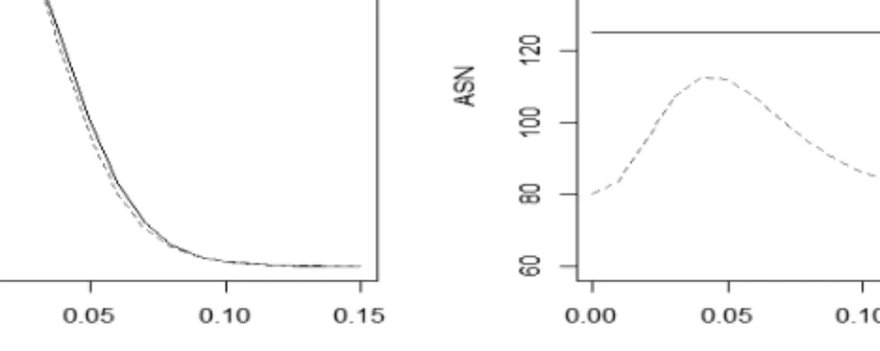
2.13 Comparison of OC and ASN Curves for ANSI/ASQ Z1.4 Single and Double Plans . . . 37

2.14 Comparison of Normal, Tightened, and Scheme OC Curves and ASN for Scheme . . . 39

3.1 AQL and RQL for Variable Plan . . . 45

3.2 Standard Normal QuantileZ_α andZ_AQL . . . 46

3.3 OC Curve for Variables Sampling Plann= 21,k= 1.967411 47 3.4 OC Curve for Attribute Sampling Plann= 172, c= 4 . . . . 49

3.5 Comparison of OC Curves for Attribute and Variable Sampling Plans . . . 51

3.6 Content of MIL-STD 414 . . . 61

3.7 Gauge R&R Plots . . . 66

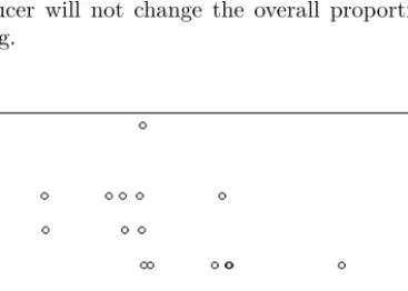
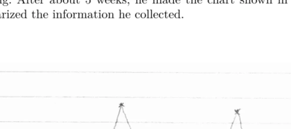
3.8 Simulated between the proportion nonconforming in a sample and the proportion nonconforming in the remainder of the lot 69 4.1 Patrick’s Chart (Source B.L. Joiner Fourth Generation Man- agement, McGraw Hill, NY, ISBN0-07032715-7) . . . 74

4.2 Control Chart of Patrick’s Data . . . 75

4.3 Coil.csv file . . . 78

xiii

(15)

4.4 R-chart for Coil Resistance . . . 80

4.5 X-chart for Coil Resistance . . . 80

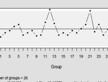
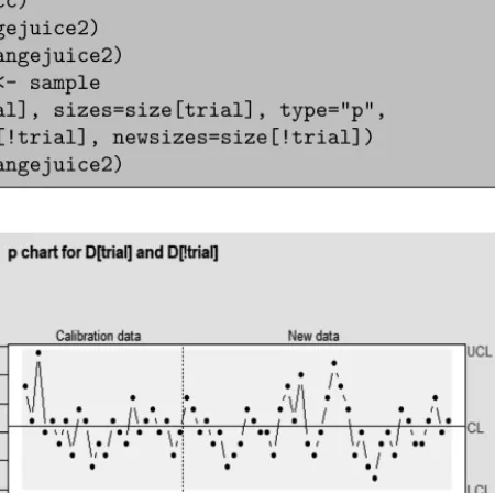
4.6 pchart of the number nonconforming . . . 86

4.7 Revised limits with additional subgroups . . . 87

4.8 OC Curve . . . 88

4.9 Flowchart Symbols . . . 93

4.10 Creating a Flowchart . . . 94

4.11 PDCA or Shewhart Cycle . . . 95

4.12 Cause-and-Effect-Diagram Major Categories . . . 97

4.13 Cause-and-Effect-Diagram–First Level of Detail . . . 97

4.14 Cause-and-Effect-Diagram–Second Level of Detail . . . 98

4.15 qcc Cause-and-Effect Diagram . . . 99

4.16 Defective Item Check Sheet . . . 100

4.17 Standard Deviations of Plaque Potency Assays of a Reference Standard . . . 102

4.18 Pareto Chart of Noconforming Cans Sample 23 . . . 103

4.19 Scatter Plot of Cycle Time versus Yield . . . 104

4.20 Scatter Plot of Cycle Time versus Contamination Defects . . 105

4.21 Capability Analysis of Lathe Data in Table 4.3 . . . 108

4.22 OC curves for Coil Data . . . 111

4.23 OC curves for Coil Data . . . 111

4.24 ARL curves for Coil Data with Hypothetical Subgroup Sizes of 1 and 5 . . . 112

4.25 OC curves for Orange Juice Can Data, Subgroup Size=50 . . 113

4.26 CE Diagram for exercise . . . 115

5.1 SIPOC Diagram . . . 121

5.2 Symbolic representation of a 2³Design . . . 125

5.3 Representation of the Effect of Factor A . . . 126

5.4 Conditional Main Effects of B given the level of C . . . 127

5.5 BC interaction effect . . . 128

5.6 BC Interaction Plot . . . 132

5.7 Model Diagnostic Plots . . . 133

5.8 Normal Plot of Coefficients . . . 136

5.9 AC Interaction Plot . . . 137

5.10 CD Interaction Plot . . . 138

5.11 Tunnel Kiln . . . 143

5.12 Caption . . . 144

5.13 Tile Manufacturing Process . . . 144

5.14 Normal Plot of Half-Effects . . . 147

5.15 CD Interaction Plot . . . 147

5.16 Normal Plot of Effects from Ruggedness Test . . . 152

5.17 CF Interaction Plot . . . 153

5.18 CE Interaction Plot . . . 157

5.19 Quadratic Response Surface . . . 159

(16)

5.20 Central Composite Design . . . 159

5.21 Sequential Experimentation Strategy . . . 161

5.22 Contour Plots of Fitted Surface . . . 167

6.1 Individuals Chart of Random Data . . . 174

6.2 Plot of Cumulative Sums of Deviations from Table 6.1 . . . . 175

6.3 Standardized Cusum Chart of the Random Data in Table 6.1 withk= 1/2 andh= 5 . . . 177

6.4 EWMA for Phase II Data from Table 6.5 . . . 184

6.5 Cusum Chart of vi . . . 190

6.6 Cusum Chart of yi . . . 190

6.7 EWMA Charts ofyi and vi . . . 192

6.8 CaptionSimulated Distribution of R/d₂σ . . . 193

6.9 EWMA chart of Simulated Phase II Data with AdjustedL . 197 6.10 EWMA chart ofvifrom Simulated Phase II Data with Adjusted L . . . 197

6.11 Normal Approximation to Poisson withλ= 2 andcchart control limits . . . 198

6.12 Wire Pull Failure Modes . . . 200

6.13 Cusum for counts without and with FIR . . . 204

7.1 Comparison of Elliptical and Independent Control . . . 210

7.2 Phase IT² Chart . . . 216

7.3 Ellipse Plot Identifying Out-of-control Subgroups . . . 217

7.4 Phase IT² Chart Eliminating Subgroups 10 and 20 . . . 218

7.5 Ellipse Plot Identifying Out-of-control Subgroup 6 . . . 219

7.6 Phase IT² Chart Eliminating Subgroups 6, 10, and 20 . . . . 220

7.7 Control Chart of Generalized Variances |S| for Ryan’s Table 9.2 223 7.8 Control Chart of Generalized Variances |S| for dataframe Frame 225 7.9 T² Control Chart of Subgroup Mean Vectors in dataframe Frame . . . 226

7.10 Control Chart of Generalized Variances |S| for dataframe Frame Eliminating Subgroup 10. . . 227

7.11 T² Control Chart of Subgroup Mean Vectors in dataframe Frame after Eliminating Subgroup 10 . . . 229

7.12 Phase IIT² Chart with 20 New Subgroups of Data . . . 230

7.13 Phase IT² Chart of Drug Impurities . . . 232

7.14 Phase I T²Chart of Drug Impurities after Eliminating Obser- vation 8 . . . 233

7.15 Phase I T²Chart of Drug Impurities after Eliminating Obser- vation 8, and 4 . . . 234

7.16 Phase IIT² Chart of Drug Impurities . . . 235

7.17 Barchart of Impurity Percentage Changes from the Mean for Observation . . . 236

7.18 MEWMA Chart of Randomly Generated Data D . . . 241

(17)

7.19 T² Chart of Randomly Generated Data D . . . 242

8.1 Quality Manual Documentation Tiers . . . 249

8.2 Flowchart of ISO 9000 Registration Process . . . 252

8.3 Malcolm Baldrige Quality Award Organization . . . 254

8.4 Motorola Six Sigma Concept . . . 258

8.5 Six Sigma Organization . . . 260

8.6 DMAIC Process . . . 260

(18)

1.1 ISO 9001 Registrations by Country 2014 . . . 8

2.1 A Multiple Sampling Plan . . . 21

2.2 A Multiple Sampling Plan with k=6 . . . 22

2.3 The ANSI/ASQ Z1.4 Double Sampling Plan . . . 40

2.4 The ANSI/ASQ Z1.4 Multiple Sampling Plan . . . 41

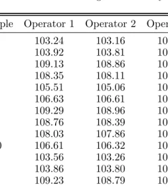
3.1 Results of Gauge R&R Study . . . 64

3.2 Average Sample Numbers for Various Plans . . . 68

4.1 Coil Resistance . . . 79

4.2 PDCA and the Scientific Method . . . 96

4.3 Groove Inside Diameter Lathe Operation . . . 106

4.4 Capability Indices and Process Fallout in PPM . . . 109

4.5 Phase I Study for Bend Clip Dim "A" (Specification Limits .50 to .90 mm) . . . 116

5.1 Factors and Levels in Nickel-Cadmium Battery Assembly Ex- periment . . . 129

5.2 Factor Combinations and Response Data for Battery Assembly Experiment . . . 130

5.3 Factors and Levels for Injection Molding Experiment . . . 134

5.4 Factor Combinations and Response Data for Injection Molding Experiment . . . 134

5.5 Fractional Factorial by Random Elimination . . . 139

5.6 Fractional Factorial by Confounding E and ABCD . . . 140

5.7 Factors and Levels in Robust Design Experiment . . . 145

5.8 List of Experiments and Results for Robust Design Experiment 145 5.9 Factors and Levels in Ruggedness Experiment . . . 149

5.10 Factors and Levels in Spin-Coater Experiment . . . 155

5.11 List of Runs for Central Composite Design in 3 Factors . . . 160

5.12 Number of runs for Central Composite Design . . . 161

5.13 Factors and Uncoded Low and High Levels in Mesoporus Car- bon Experiment . . . 163

6.1 Cumulative Sums of Deviations from the Mean . . . 175

6.2 Standardized Tabular Cusums . . . 177 xvii

(19)

6.4 ARL for Shewhart and Cusum Control Charts . . . 180 6.5 EWMA Calculations λ= 0.2 Phase II Data from Table 6.3 . 183 6.6 ARL for Shewhart and Cusum Control Charts and EWMA

Charts . . . 185 6.7 Expected value ofp

|yi| andv_i as function ofγ . . . 186 6.8 ARL for Detecting Increases inσby Monitoring v_i . . . 188 6.9 ARL for Various Values of hwithk= 2,λ₀= 1.88 . . . 201 6.10 Calculations for Counted Data Cusum for Detecting an Increase

withk= 2,h= 10 . . . 202 6.11 Comparison of ARL for cchart and Cusum for Counted Data

(k= 5,h= 10) with Targetλ= 4 . . . 203 7.1 Upper control limitsh₄for MEWMA Charts with r=.1 . . . 238 7.2 ARL Comparisons between T² and MEWMA Charts–note:

Source Lowry et. al.Technometrics 34:46-53, 1992 . . . 243 8.1 Motorola Six Sigma % and ppm out of Spec . . . 258

(20)

Introduction and Historical Background

Statistical Quality Control includes both (1) the application of statistical sampling theory that deals with quality assurance and (2) the use of statistical techniques to monitor and control a process. The former includes acceptancesampling procedures for inspecting incoming parts or raw materials, and the latter (often referred to as statistical process control or SPC) employs the use of control charts, continuous improvement tools, and the design of experiments for early detection and prevention of problems, rather than correction of problems that have already occurred.

1.1 Origins of Statistical Quality Control

Quality control is as old as industry itself, but the application of statistical theory to quality control is relatively recent. When AT&T was developing a nationwide telephone system at the beginning of the 20th century, sampling inspection was used in some form at the Western Electric Company (the AT&T equipment manufacturing arm). Also, according to an article in theGeneral Electric Review in 1922, some formal attempts at scientific acceptance sampling techniques were being made at the G.E. Lamp Works.

At Western Electric, an Inspection Engineering Department was formed, which later became the Quality Assurance Department of the Bell Telephone Laboratories. In 1924, Walter Shewhart, a physicist and self-made statistician, was assigned to examine and interpret inspection data from the Western Electric Company Hawthorn Works. It was apparent to him that little useful inference to the future could be drawn from the records of past inspection data, but he realized that something serious should be done and he conceived the idea of statistical control. It was based on the premise that no action can be repeated exactly. Therefore, all manufactured product is subject to a cer- tain amount of variation that can be attributed to a system of chance causes.

Stable variation within this system is inevitable. However, the reasons for special cause variation outside this stable pattern can (and should) be recognized and eliminated.

The control chart he perceived was founded on sampling during production rather than waiting until the end of the production run. Action limits were 1

(21)

calculated from the chance cause variation in the sample data, and the process could be immediately stopped and adjusted when additional samples fell outside the action limits. In that way, production output could be expected to stay within defined limits.

The early dissemination of these ideas was limited to the circulation of memos within the Bell Telephone System. However, the soundness of the pro- posed methods was thoroughly validated by staff at Western Electric and the Bell Telephone Laboratories. The methods worked effectively and were soon made part of the regular procedures of the production divisions. Shewhart’s ideas were eventually published in his 1931 book The Economic Control of Quality of Manufactured Product [86].

W. Edwards Deming from the U.S. Department of Agriculture and the Census Bureau, who developed the sampling techniques that were first used in the 1940 U.S. Census, was introduced to Shewhart in 1927. He found great inspiration in Shewhart’s theory of chance (that he renamed common) and special causes of variation. He realized these ideas could be applied not only to manufacturing processes but also to administrative processes by which en- terprises are led and managed. However, many years later in a videotaped lecture Deming said that while Shewhart was brilliant, he made things ap- pear much more difficult than necessary. He therefore spent a great deal of time copying Shewhart’s ideas and devising simpler and more easily under- stood ways of presenting them.

Although Shewhart’s control charts were effective in helping organizations control the quality of their own manufacturing processes, they were still dependent on the quality of raw materials, purchased parts and the prevailing quality control practices of their suppliers. For these reasons, sampling inspection of incoming parts remained an important part of statistical quality control.

Harold F. Dodge joined Western Electric Corporation shortly after She- whart did. He wondered, “how many samples were necessary when inspecting a lot of materials”, and began developing sampling inspection tables. When he was joined by Harry G. Romig, together they developed double sampling plans to reduce the average sample size required, and by 1927 they had developed tables for rectification inspection indexed by the lot tolerance and AOQL (average outgoing quality level). Rectification sampling required re- moval of defective items through 100% inspection of lots in which the number defective in the sample was too high. Dodge and Romig’s sampling tables were published in theBell System Technical Journal in 1941 [24].

The work of Shewhart, Dodge and Romig at Bell Telephone constituted much of the statistical theory of quality control at that time. In the 1930s, the Bell System engineers who developed these methods sought to popularize them in cooperation with the American Society for Testing and Materials, the American Standards Association, and the American Society of Mechanical Engineers. Shewhart also traveled to London where he met with prominent British statisticians and engineers.

(22)

Despite attempts to publicize them, adoption of statistical quality control in the United States was slow. Most engineers felt their particular situation was different and there were few industrial statisticians who were adequately trained in the new methods. By 1937, only a dozen or more mass production industries had implemented the methods in normal operation. There was much more rapid progress in Britain, however. There, statistical quality control was being applied to products such as coal, coke, textiles, spectacle glass, lamps, building materials, and manufactured chemicals (see Freeman[30]).

1.2 Expansion and Development of Statistical Quality Control during WW II

The initial reluctance to adopt statistical quality control in the United States was quickly overcome at the beginning of World War II. Manufacturing firms switched from the production of consumer goods to defense equipment. With the buildup of military personnel and material, the armed services became large consumers of American goods, and they had a large influence on quality standards.

The military had impact on the adoption of statistical quality control methods by industry in two different ways. The first was the fact that the armed services themselves adopted statistically derived sampling and inspection methods in their procurement efforts. The second was the establishment of a widespread educational program for industrial personnel at the request of the War Department.

Sampling techniques were used at the Picatinney Arsenal as early as 1934 under direction of L. E. Simon. In 1936, the Bell Telephone Laboratories were invited to cooperate with the Army Ordnance Department and the American Standards Association Technical Committee in developing war standards for quality control. In 1942, Dodge and Romig completed the Army Ordnance Standard Sampling Inspection Tables, and the use of these tables was introduced to the armed services through a number of intensive training courses.

The Ordnance Sampling Inspection Tables employed a sampling scheme based on an acceptable quality level (AQL). The scheme assumed that there would be a continuing stream of lots submitted by a supplier. If the supplier’s quality level was worse than the AQL, the scheme would automatically switch to tightened inspection and the supplier would be forced to bear the cost of a high proportion of lots rejected and returned. This scheme encouraged suppliers to improve quality.

In 1940, the military established a widespread training program for industrial personnel, most notably suppliers of military equipment. At the request of the War Department, the American Standards Association developed American War Standards Z1.1-1941 and Guide for Quality Control Z.1-2-1941, Control Chart Method of Analyzing Data–1941, and the Control Chart

(23)

Method of Controlling Quality during Production Z1.3-1942. These defined the American control chart practice and were used as the text material for subsequent training courses that were developed at Stanford by Holbrook Working, E. L. Grant, and W. Edwards Deming. In 1942 this intensive course on statistical quality control was given at Stanford University to representa- tives of the war industries and procurement agencies of the armed services.

The early educational program was a success. That success, along with the suggestion from Dr. Walter Shewhart that Federal assistance should be given to American war industries in developing applications of statistical quality control, led the Office of Production and Research and Development (OPRD) of the War Production Board to establish a nationwide program. The program combined assistance in developing intensive courses for high ranking executives from war industry suppliers and direct assistance to establishments on specific quality control problems. The specific needs to be addressed by this program for the war-time development of statistical quality control were:

1. Education of industrial executives regarding the basic concepts and benefits of statistical quality control.

2. Training of key quality control personnel in industry.

3. Advisory assistance on specific quality control problems.

4. Training of subordinate quality control personnel.

5. Training of instructors.

6. Publication of literature.

The training of instructors was regarded as an essential responsibility of the OPRD program. The instructors used were competent and experienced university teachers of statistics who only needed to (1) extend their knowledge in in the specific techniques and theory most relevant to statistical quality control, (2) become familiar with practical applications, and (3) learn the instructional techniques that had been found to be most useful.

The plan was to have courses for key quality control personnel from industry given at local educational institutions, which would provide an instructor from their own staff. This plan was implemented with administrative assistance and grants from the Engineering, Science and Management War Train- ing Program (ESMWT) funded by the U.S. Office of Education.

Much of the training of subordinate quality control personnel was given in their own plants by those previously trained. To stimulate people to actively advance their own education, the OPRD encouraged local groups to form.

That way neighboring establishments could exchange information and expe- riences. These local groups resulted in the establishment of many regional quality control societies. The need for literature on statistical quality control was satisfied by publications of the American Standards Association and articles in engineering and technical journals.

(24)

As a result of all the training and literature, statistical quality control techniques were widely used during the war years. They were instrumental in ensuring the quality and cost effectiveness of manufactured goods as the na- tions factories made the great turnaround from civilian to military production.

For example, military aircraft production totaled 6000 in 1940 and jumped to 85,000 in 1943. Joseph Stalin stated that without the American production, the Allies could never have won the war.

At the conclusion of the War in 1946, seventeen of the local quality control societies formed during the war organized themselves into the American Soci- ety for Quality Control (ASQC). This society has recently been renamed the American Society for Quality (ASQ) to reflect the fact that Quality is essential to much more than manufacturing firms. It is interesting to note that outside the board room of ASQ in Milwaukee Wisconsin stands an exhibit memori- alizing W.E. Deming’s famous Red Bead Experiment¹ (a teaching tool) that was used during the war effort to show managers the futility of the standard reaction to common causes of variation.

The development and use of sampling tables and sampling schemes for military procurement continued after the war, resulting in the MIL-STD 105A attributes sampling scheme, which was later revised as 105B, 105C, 105D, and 105E. In addition, variables sampling schemes were developed that eventually resulted in MIL-STD 414.

1.3 Use and Further Development of Statistical Quality Control in Post-War Japan

After the war, companies that had been producing defense equipment resumed producing goods for public consumption. Unfortunately, the widespread use of statistical quality control methods that had been used so effectively in producing defense equipment did not carry over into the manufacture of civilian goods. Women who filled many positions in inspection and quality improvement departments during the war left the workforce and were replaced by military veterans who were not trained in the vision and technical use of SPC. Industry in Europe lay in the ruins of war, and the overseas and domestic demand for American manufactured goods exceeded the supply. Because they could sell everything they produced, company top managers failed to see the benefits of the extra effort required to improve quality. As the U. S. economy grew in the 1950s there were speculations of a coming recession, but it never came. The demand for products continued to increase leaving managers to believe they were doing everything right.

1This was used to teach the futility of reacting to common cause variation by making changes to the process, and the need for managers to understand the system before placing unreasonable piecework standards upon workers—see https://www.youtube.com/watch?v=ckBfbvOXDvU

(25)

At the same time, U.S. occupation forces were in Japan trying to help rebuild their shattered economy. At the request of General Douglas McArthur, W. E. Deming was summoned to help in planning the 1951 Japan Census.

Deming’s expertise in quality control techniques and his compassion for the plight of the Japanese citizens brought him an invitation by the Japanese Society of Scientists and Engineers (JUSE) to speak with them about SPC.

At that time, what was left of Japanese manufacturing was almost worse than nothing at all. The label Made in Japan was synonymous with cheap junk in worldwide markets.

Members of JUSE had been interested in Shewhart’s ideas and they sought an expert to help them understand how they could apply them in the re- construction of their industries. At their request, Deming, a master teacher, trained hundreds of Japanese academics, engineers, and managers in statistical quality control techniques. However, he was troubled by his experience in the United States where these techniques were only widely used for a short time during the war years. After much speculation, Deming had come to the conclusion that in order for the use of these statistical techniques to endure, a reputable and viable management philosophy was needed that was consis- tent with statistical methods. As a result Deming developed a philosophy that he called the 14 Points for Management. There were originally less than 14 points, but they evolved into 14 with later experience.

Therefore, when Deming was invited by JUSE to speak with them about SPC, he agreed to do so only if he could first talk directly to top management of companies. In meetings with executives in 1950, his main message was his Points for Management² and the following simple principle: (1) Improve

2https://asq.org/quality-resources/total-quality-management/deming-points

1. Create constancy of purpose for improving products and services.

2. Adopt the new philosophy.

3. Cease dependence on inspection to achieve quality.

4. End the practice of awarding business on price alone; instead, minimize total cost by working with a single supplier.

5. Improve constantly and forever every process for planning, production and service.

6. Institute training on the job.

7. Adopt and institute leadership.

8. Drive out fear.

9. Break down barriers between staff areas.

10. Eliminate slogans, exhortations and targets for the workforce.

11. Eliminate numerical quotas for the workforce and numerical goals for management.

12. Remove barriers that rob people of pride of workmanship, and eliminate the annual rating or merit system.

13. Institute a vigorous program of education and self-improvement for everyone.

14. Put everybody in the company to work accomplishing the transformation.

(26)

Quality ⇒(2) Less Rework and Waste ⇒ (3) Productivity Improves ⇒ (4) Capture the Market with Lower Price and Better Quality⇒(5) Stay in Busi- ness⇒(6) Provide Jobs.

With nothing to lose, the Japanese manufactures applied the philosophy and techniques espoused by Deming and other American experts in Qual- ity. The improved quality, along with lower cost of the goods, enabled the Japanese to create new international markets for Japanese products, espe- cially automobiles and consumer electronics. Japan rose from the ashes of war to becoming one of the largest economies in the world. When Deming declined to accept royalties on the published transcripts of his 1950 lectures, the JUSE board of directors used the proceeds to establish the Deming Prize, a silver medal engraved with Demings profile. It is given annually in a nationally tele- vised ceremony to an individual for contributions in statistical theory and to a company for accomplishments in statistical application.

As Deming predicted in 1950, Japanese products gained respect in worldwide markets. In addition, Japanese began to contribute new insights to the body of knowledge regarding SQC. Kaoru Ishikawa, a Deming Prize recipient, developed the idea of quality circles where foreman and workers met together to learn problem solving tools and apply them to their own process. This was the beginning of participative management. Ishikawa also wrote books on quality control including hisGuide to Quality Control that was translated to English and defined the 7 basic quality tools to be discussed later inChapter 4. Genichi Taguchi developed the philosophy of off-line quality control where products and processes are designed to be insensitive to common sources of variation that are outside the design engineers control. An example of this will be shown inChapter 5.

When the Arab Oil Embargo caused the price of oil to increase from $3 to $12 per barrel in 1973, it created even more demand for small fuel-efficient Japanese cars. In the U.S, when drivers began to switch to the smaller cars, they noticed that in addition to being more fuel efficient, they were more reliable and less problematic. By 1979, U.S. auto manufactures had lost a major share of their market, and many factories were closed and workers laid off. This was a painful time, and when the NBC Documentary "If Japan Can, Why Can’t We" aired in 1979, it was instrumental in motivating industry lead- ers to start re-learning the quality technologies that that had helped Japan’s manufacturing, but were in disuse in the U.S.

1.4 Re-emergence of Statistical Quality Control in U.S.

and the World

Starting about 1980, top management of large U.S. Companies began to accept quality goals as one of the strategic parameters in business planning along

(27)

with the traditional marketing and financial goals. For example, Ford Motor Company adopted the slogan "Quality is Job 1", and they followed the plan of the Defense department in WW II by setting up training programs for their own personnel and for their suppliers. Other companies followed suit, and the quality revolution began in the U.S.

Total Quality Management or TQM was adopted by many U.S companies.

This management system can be described as customer focused and involves all employees in continual improvement efforts. As described on the American Society for Quality (ASQ) website³"It uses strategy, data, and effective com- munications to integrate the quality discipline into the culture and activities of the organization".

Based on efforts like this, market shares of U.S. companies rebounded in manufactured goods such as automobiles, electronics, and steel. In addition, the definition of Quality expanded from just meeting manufacturing specifi- cations to pleasing the customer. The means of providing quality through the expanded definition of SQC as espoused by Deming and others was adopted in diverse areas such as utility companies, health care institutions, banking and other customer service organizations.

A worldwide movement began using the same philosophy. In 1987, the International Standardization Organization created the Standards for Quality Assurance Systems (ISO 9000). It was the acknowledgement of the worldwide acceptance of the systems approach to producing Quality. ISO 9001 deals with the requirements that organizations wishing to meet the standard must fulfil.

Certification of compliance to these standards are required for companies to participate in the European Free Trade Association (EFTA).Table 1.1shows the number of companies ISO 9001 registered by country.

TABLE 1.1

ISO 9001 Registrations by Country 2014

Rank Country ISO 9001 Registrations

1 China 342,180

2 Italy 168,960

3 Germany 55,563

4 Japan 45,785

5 India 41,016

6 United Kingdom 40,200

7 Spain 36,005

8 United States 33,008

9 France 29,122

10 Austria 19,731

In 1988, the U.S. Congress established the Malcolm Baldrige National Quality Award named after the late secretary of commerce. This is similar to the Deming award in Japan, and it was a recognition by the U.S. government

3https://asq.org/quality-resources/total-quality-management

(28)

of the need to focus on the quality of products and services in order to keep the U.S. economy competitive.

Other changes to statistical quality control practices have also taken place.

The U. S. Department of Defense discontinued support of their Military Stan- dards for Sampling Inspection in order to utilize civilian standards as a cost savings. The ANSI/ASQ Z1.4 is the civilian standard in the U.S. that replaces the MIL-STD 105E Attribute Sampling Inspection Tables. It is best used for domestic transactions or in-house use. The ISO 2851-1 is the international standard. It reflects the current state of the art and is recommended for international trade, where it is often required. The U.S. civilian standard to replace MIL-STD 414 Variables Sampling Plans is ANSI/ASQ Z1.9. It was designed to make the inspection levels coincide with the Z1.4 plans for attributes and adopts common switching rules. ISO 3951-1 is the international version with plans closely matched to the ISO 2851-attribute plans. It is also used in international trade.

Another change in the application of technical methodologies for quality control and quality improvement is the use of the computer. Prior to 1963, the only tools available to engineers and statisticians for calculations were slide rules or mechanical or electro-mechanical calculators. Sampling inspection tables and Shewhart’s control charts were developed with this fact in mind.

After availability of computers, software began to be developed for statistical calculations and SQC applications. However, much of the training materials and textbooks that have been developed since the 1980 comeback of SQC in U.S. industry still illustrates the techniques that can easily be implemented with hand calculations. However, this book will emphasize the use of the computer for SQC calculations.

Popular commercial software used in industry includes programs such as SynergySPC and SQCpack that can share data and reports between different computers. Others like SAS, Minitab 18, or StatGraphics Centurion combine SQC calculations with data manipulation features and a full suite of statistical analysis tools.

This book will illustrate the use of R, since it is a free programming language and environment for statistical computing. R was developed by Ross Ihaka and Robert Gentleman at the University of Auckland, New Zealand.

It implements the S programming language that was developed at Bell Labs by John Chambers in 1976. R is highly extendible through functions and ex- tensions. There are many user written packages for statistical quality control functions that are available on the Comprehensive Archive Network (CRAN).

(29)

(30)

Attribute Sampling Plans

2.1 Introduction

The quality and reliability of manufactured goods are highly dependent on the quality of component parts. If the quality of component parts is low, the quality and/or reliability of the end assembly will also be low. While some component parts are produced in house, many are procured from outside suppliers; the final quality is, therefore, highly dependent on suppliers.

In response to stiff competition, Ford Motor Company adopted procedu- ral requirements for their suppliers in the early 1980s to insure the quality of incoming component parts. They demanded that all their suppliers show that their production processes were in a state of statistical control with a capability index greater than 1.5. Because Ford Motor Company bought such a large quantity of component parts from their suppliers, they were able to make this demand.

Smaller manufacturing companies may not have enough influence to make similar demands to their suppliers, and their component parts may come from several different suppliers and sub-contractors scattered across different countries and continents. However, by internal use of acceptance sampling procedures, they can be sure that the quality level of their incoming parts will be close to an agreed upon level. This chapter will illustrate how the AcceptanceSampling and AQLSchemes packages in R can be used both to create attribute sampling plans and sampling schemes and evaluate them.

2.2 Attribute Data

When numerical measurements are made on the features of component parts received from a supplier, quantitative data results. On the other hand, when only qualitative characteristics can be observed, attribute data results. If only attribute data is available, incoming parts can be classified as either conforming/nonconforming, non-defective/defective, pass/fail, or present/absent etc. Attribute data also results from inspection data (such as inspection of billing records), or the evaluation of the results of maintenance operations or 11

(31)

administrative procedures. Non conformance in these areas is also costly. Er- rors in billing records result in delayed payments and extra work to correct and resend the invoices. Non conformance in maintenance or administrative procedures, result in rework and less efficient operations.

2.3 Attribute Sampling Plans

A lot or Batch is defined as "a definite quantity of a product or material accumulated under conditions that are considered uniform for sampling pur- poses" [6]. The only way that a company can be sure that every item in an incoming lot of components from a supplier, or every one of their own records or results of administrative work completed, meets the accepted standard is through 100% inspection of every item in the lot. However, this may require more effort than necessary, and if the inspection is destructive or damaging, this approach cannot be used.

Alternatively, a sampling plan can be used. When using a sampling plan, only a random sample of the items in a lot is inspected. When the number of nonconforming items discovered in the sample of inspected components is too high, the lot is returned to the supplier (just as a customer would return a defective product to the store). When inspecting the records of administrative work completed, and the number of nonconforming records or nonconforming operations are too high in a lot or period of time, every item in that period may be inspected and the work redone if nonconforming. On the other hand, if the number of nonconforming items discovered in the sample is low, the lot is accepted without further concern.

Although a small manufacturing company may not be able to enforce pro- cedural requirements upon their suppliers, the use of an acceptance sampling plan will motivate suppliers to meet the agreed upon acceptance quality level or improve their processes so that it can be met. Otherwise, they will have to accept returned lots which will be costly.

When inspecting only a random sample from a lot, there is always a non- zero probability that there are nonconforming items in the lot even when there are no nonconforming items discovered in the sample. However, if the customer and supplier can agree on the maximum proportion nonconforming items that may be allowed in a lot, then an attribute acceptance sampling plan can be used successfully to reject lots with proportion nonconforming above this level.

The sampling plan can both maximize the probability of rejecting lots with a higher proportion nonconforming than the agreed upon level (benefit to the customer), and it can maximize the probability of accepting lots that have the proportion nonconforming at or below the agreed upon level (benefit to the supplier).

(32)

For a lot of N components, an attribute sampling plan consists of the number of items to be sampled,n, and the acceptance number or maximum number of nonconforming items,c, that can be discovered in the sample and still allow the lot to be accepted. The probability of accepting lots with varying proportions of nonconforming or defective items using an attribute acceptance sampling plan can be represented graphically by the OC (or Operating Char- acteristic) curve shown inFigure 2.1.

FIGURE 2.1: Operating Characteristic Curve

In this figure the AQL (Acceptance Quality Level) represents the agreed upon maximum proportion of nonconforming components in a lot. 1−αrep- resents the probability of accepting a lot with the AQL proportion nonconforming, and the PR=αis the producer’s risk or probability that a lot with AQL proportion nonconforming is rejected. The IQ is the indifference quality level where 50% of the lots are rejected, and RQL is the rejectable quality level where there is only a small probability, β, of being accepted. The customer should decide on the RQL. CR=β is the customer’s risk.

From the customer’s point of view, a steeper OC curve with a smaller operating ratio (or ratio of the RQL to the AQL) is preferable. In this case, the probability of accepting any lot with greater than the AQL proportion nonconforming is reduced. To prevent rejected lots, the supplier will be motivated to send lots with the proportion nonconforming less than the AQL. The ideal OC curve is shown inFigure 2.2. It would result when 100% inspection is used or n =N and c=AQL×N. In this case, all lots with a proportion nonconforming (or defective) less than the AQL are accepted, and all lots with the proportion nonconforming greater than the AQL are rejected. As the fraction

(33)

items sampled (n/N) in a sampling plan increases, the OC curve for that plan will approach the curve for the ideal case.

FIGURE 2.2: Ideal Operating Characteristic Curve for a Customer

Experience with sampling plans has led to the standard values of α=PR=0.05 and β=CR=0.10 according to Schilling and Neubauer[84]. This will result in one lot in 20 rejected when proportion nonconforming is at the AQL, and only one lot in 10 accepted when the proportion nonconforming is at the RQL. When β=0.10, the RQL is usually referred to as the LTPD or Lot Tolerance Percent Defective. Whileα =.05 and β = 0.10 are common, other values can be specified. For example, if nonconforming items are costly then it may be desirable to use a β less than 0.10, and if rejecting lots that have the AQL proportion nonconforming is costly, it may be desirable to use αless than 0.05.

2.4 Single Sample Plans

In a single sampling plan, as described in the last section, allnsample units are collected before inspection or testing starts. Single sampling plans specify the number of items to be sampled,n, and the acceptance number,c. Single sampling plans can be obtained from published tables such as MIL-STD- 105E, ANSI/ASQ Standard Z1.4, ASTM International Standard E2234, and ISO Standard 2859. Plans in these published tables are indexed by the lot

(34)

size and AQL. The tables are most useful for the case when a purchaser buys a continuing stream of lots or batches of components, and the purchaser and seller agree to use the tables. More about these published sampling plans will be discussed inSection 2.6.

Custom derived sampling plans can be constructed for inspecting isolated lots or batches. Analytic procedures have been developed for determining the sample size, n, and the acceptance number, c, such that the probability of accepting a lot with the AQL proportion nonconforming will be as close as possible to 1−α, and the probability of accepting a lot with RQL proportion nonconforming will be as close as possible toβ. These analytic procedures are available in thefind.plan()function in the R packageAcceptanceSampling that can be used for finding single sampling plans.

As an example of this function, consider finding a sampling plan where the AQL=0.05,α=.05, RQL = 0.15, andβ=0.20 for a lot of 500 items. For a plan where the sample size isnand the acceptance number isc, the probability of accepting a lot ofN=500 withD nonconforming or defective items is given by the cumulative Hypergeometric distribution, i.e.,

P r(accept) =

c

X

i=0

D i

N−D n−i

N

n

(2.1)

Thefind.plan()function attempts to findnandcso that the probability of accepting whenD= 0.05×N is as close to 1−0.05 =.95 as possible, and the probability of accepting when D= 0.15×N is as close to 0.20 as possible. The first statement in the R code below loads theAcceptanceSampling package. The next statement is the call tofind.plan(). The first argument in the call,PRP=c(0.05,0.95), specifies the producer risk point (AQL, 1−α);

the second argument specifies the consumer risk point (RQL,β); the next argument,type="hypergeom", specifies that the probability distribution is the hypergeometric; and the last argument,N=500, specifies the lot size.

R>library(AcceptanceSampling)

R>find.plan(PRP=c(0.05,0.95),CRP=c(0.15,0.20), type="hypergeom",N=500)

In the output below we see that the sample size should be n=51 and the acceptance numberc= 5.

(35)

$n [1] 51

$c [1] 5

$r [1] 6

The following code produces the OC curve for this plan that is shown in Figure 2.3.

R>plan<-OC2c(51,5,type="hypergeom", N=500, pd=seq(0,.25,.01)) R>plot(plan, type=’l’)

R>grid()

FIGURE 2.3: Operating Characteristic Curve for the plan with N = 500, n= 51, andc= 5

The code below shows how to determine how close the producer and consumer risk points for this plan are to the requirement.

R>assess(OC2c(51,5), PRP=c(0.05, 0.95), CRP=c(0.15,0.20)) The output shows the actual probability of acceptance at AQL is 0.9589 and the probability of acceptance at RQL is 0.2032.

(36)

Acceptance Sampling Plan (binomial) Sample 1

Sample size(s) 51

Acc. Number(s) 5

Rej. Number(s) 6

Plan CANNOT meet desired risk point(s):

Quality RP P(accept) Plan P(accept)

PRP 0.05 0.95 0.9589318

CRP 0.15 0.20 0.2032661

To make the OC curve steeper and closer to the customer’s ideal, the required RQL can be made closer to the AQL. For example in the R code below, the RQL is reduced from 0.15 to 0.08. As a result, the find.plan function finds a plan with a much higher sample sizen= 226 (nearly 50% of the lot sizeN = 500), and acceptance numberc= 15.

R>find.plan(PRP=c(0.05,0.95),CRP=c(0.08,0.20), type="hypergeom",N=500)

$n [1] 226

$c [1] 15

$r [1] 16

The OC curve for this plan is shown inFigure 2.4, and it is steeper with a reduced operating ratio. The disadvantage to this plan over the original (n= 51,c = 5) plan is the increased sample sizen= 226. The next section discusses double and multiple sampling plans that can produce a steep OC curve with a smaller average sample size than required by a single sample plan.

2.5 Double and Multiple Sampling Plans

The aim of double sampling plans is to reduce the average sample size and still have the same producer and customer risk points. A double sampling plan consists of n₁, c₁, and r₁ which are the sample size, acceptance, and rejection numbers for the first sample; n₂, c₂, andr₂, which are the sample size, acceptance number, and rejection number for the second sample.

(37)

FIGURE 2.4: Operating Characteristic Curve for the plan with N = 500, n= 226,c= 15

A double sampling plan consists of taking a first sample of size n₁. If there arec₁ or less nonconforming in the sample, the lot is accepted. If there arer₁ nonconforming or more in the sample, the lot is rejected (where r₁ ≥ c₁+ 2). If the number nonconforming in the first sample is between c₁+ 1 andr₁−1, a second sample of sizen₂ is taken. If the sum of the number of nonconforming in the first and second samples is less than or equal toc₂, the lot is accepted. Otherwise, the lot is rejected. Although there is no function in theAcceptanceSamplingpackage in R for finding double sampling plans, the assess()function and theOC2c()function can be used to evaluate a double sampling plan, and the AQLSchemes package can retrieve double sampling plans from the ANSI/ASQ Z1.4 Standard.

Consider the following example shown by Schilling and Neubauer[84]. If a single sampling plan that hasn= 134, andc= 3 is used for a lot ofN = 1000, it will have a steep OC curve with a low operating ratio. The R code below shows that there is at least a 96% chance of accepting a lot with 1% or less nonconforming, and less than an 8% chance of accepting a lot with 5% or more nonconforming.

R>plns<-OC2c(n=134,c=3,type="hypergeom", N=1000, pd=seq(0,.20,.01))

R>assess(plns,PRP=c(.01,.95),CRP=c(.05,.10))

(38)

Acceptance Sampling Plan (hypergeom) Sample 1

Sample size(s) 134

Acc. Number(s) 3

Rej. Number(s) 4

Plan CAN meet desired risk point(s):

PRP 0.01 0.95 0.96615674

CRP 0.05 0.10 0.07785287

However, the sample size (n=134) is large, over 13% of the lot size. If a double sampling plan with n₁ = 88, c₁ = 1, r₁ = 4, and n₂ = 88, c₂ = 4, r₂= 5 is used instead, virtually the same customer risk will result, and slightly less risk for the producer. This is illustrated by the R code below.

R>pln3<-OC2c(n=c(88,88),c=c(1,4),r=c(4,5),type="hypergeom", N=1000,pd=seq(0,.20,.01))

R>assess(pln3,PRP=c(.01,.95),CRP=c(.05,.10)) Acceptance Sampling Plan (hypergeom)

Sample 1 Sample 2

Sample size(s) 88 88

Acc. Number(s) 1 4

Rej. Number(s) 4 5

Plan CAN meet desired risk point(s):

PRP 0.01 0.95 0.9805612

CRP 0.05 0.10 0.0776524

In the code above, the first argument to theOC2c()function,n=c(88,88) specifies n₁ and n₂ for the double sampling plan. The second argument c=c(1,4)specifies c₁ and c₂, and the third argument r=c(4,5) specifiesr₁ and r₂. Notice that r₂ = c₂+ 1 because a decision must be made after the second sample.

The sample size for a double sampling plan will vary betweenn₁andn₁+n₂ depending on whether the lot is accepted or rejected after the first sample.

The probability of accepting or rejecting after the first sample depends upon the number of nonconforming items in the lot, therefore the average sample number (ASN) for the double sampling plan will be:

ASN =n₁+n₂×P(c₁< x₁< r₁) (2.2)

(39)

wherex₁is the number of nonconforming items found in the first sample.

The R code below createsFigure 2.5that compares the sample size for the single sampling plan with the average sample for a double sampling plan at various proportions nonconforming or defective in the lot.

R>D=seq(0,200,5) #Number nonconforming in the lot of 1000 R>pd<-D/1000 #Proportion nonconforming in the lot of 1000 R>OC1<-phyper(1, m=D, n=1000-D, k=88, lower.tail=TRUE) R>#Probability of accepting after the first sample R> R1<-phyper(3, m=D, n=1000-D, k=88, lower.tail=FALSE) R>#Probability of rejecting after the first sample R>P<-OC1+R1

R>ASN=88+88*(1-P)

R>plot(pd,ASN,type=’l’,ylim=c(5,150),xlab="Proportion nonconforming in the lot")

R>abline(134,0,lty=2)

R>text(.10,142,’single sample n=134’) R>text(.10,70,’double sample n=(88,88)’) R>grid()

FIGURE 2.5: Comparison of Sample Sizes for Single and Double Sampling Plan

From this figure it can be seen that the average combined sample size for the double sampling plan is uniformly less than the equivalent single sampling

(40)

plan. The average sample size for the double sampling plan saves most when the proportion nonconforming in the lot is less than the AQL or greater than the RQL.

The disadvantage of a double sampling plan is that they are very difficult or impossible to apply when the testing or inspection takes a long time or must be performed off site. For example, food safety and microbiological tests may take 2 to 3 days for obtaining the result.

Multiple sampling plans extend the logic of double sampling plans, by further reducing the average sample size. Multiple sampling plans can be presented in tabular form as shown inTable 2.1

If x₁ ≤ c₁ (where x₁ is the number of nonconforming items found in the first sample) the lot is accepted. If x₁ ≥ r₁ the lot is rejected, and if c₁< x₁< r₁ another sample is taken, etc.

A multiple sampling plan with a similar OC curve as a double sampling plan will have an even lower ASN curve than the double sampling plan. The multiple sampling plan shown inTable 2.2, has an OC curve that is very similar to the single (n=134, c=3) and the double sampling plan (n₁=88, n₂=88, c₁=1, c₂=4,r₁=4,r₂=5) presented above.Figure 2.6shows a comparison of their OC curves magnifying on the region where these curves are steepest. It can be seen that within the region of the AQL=0.01 and the RQL = 0.05, these OC curves are very similar. The ASN curve for the multiple sampling plan can be shown to fall below the ASN curve for the double sampling plan shown inFigure 2.5.

Although the AcceptanceSamplingpackage does not have a function for creating double or multiple sampling plans for attributes, the ANSI/ASQ Z1.4 tables discussed in Section 2.7.2 present single, double, and multiple sampling plans with matched OC curves. The single, double, and multiple sampling plans in these tables can be accessed with theAQLSchemespackage or with the [sqc online calculator](https://www.sqconline.com/). The tables also present the OC curves and ASN curves for these plans, but the same the OC and ASN curves can be obtained from theAQLSchemespackage as well.

TABLE 2.1: A Multiple Sampling Plan

Sample Samp. Si