Our website, http://mitpress.mit.edu/algorithms/, links to solutions to some of the problems and exercises. Our website, http://mitpress.mit.edu/algorithms/, links to solutions to some of the problems and exercises so you can check your work.
Algorithms
Each nail around which the rubber band makes a turn is a vertex of the convex hull. Any of the 2n subsets of the points can be the vertices of the convex hull.
Algorithms as a technology
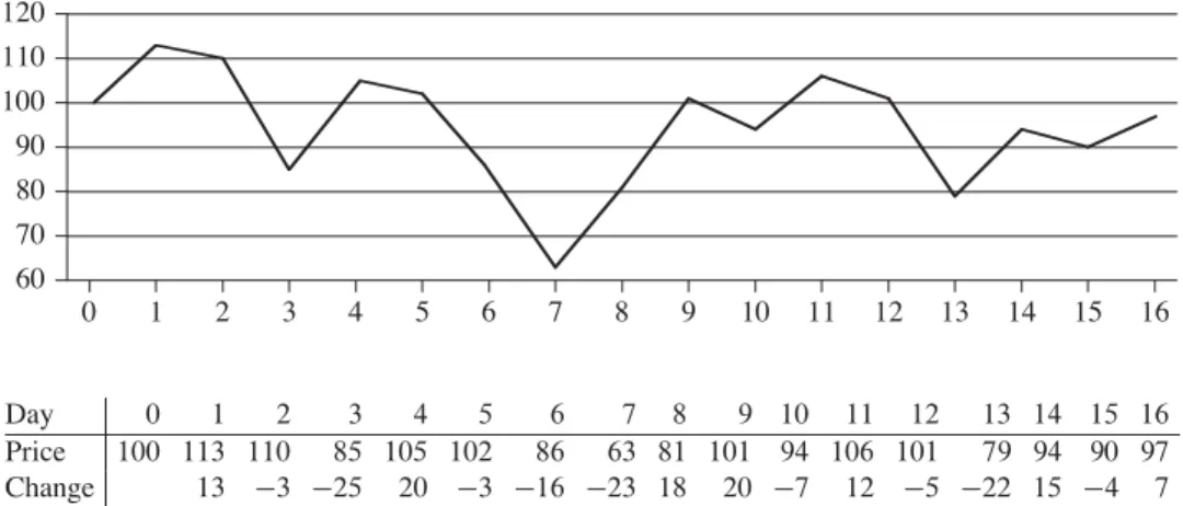
Suppose we compare implementations of insertion sort and merge sort on the same machine. For inputs of size, insertion sort runs in 8n2steps, while merge sort runs in 64nlgn steps.
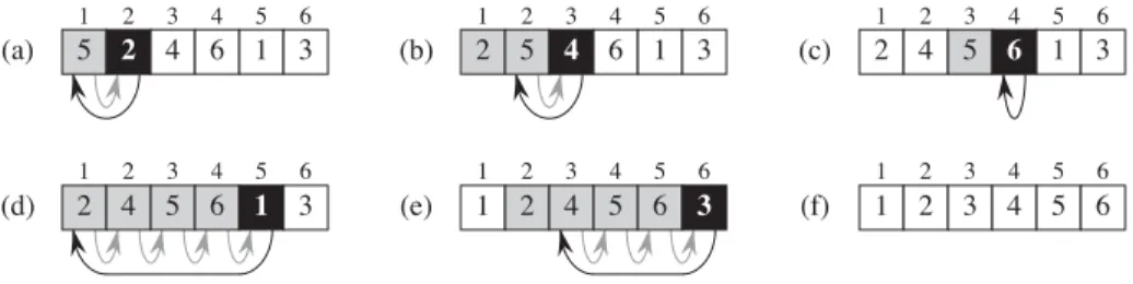
Insertion sort
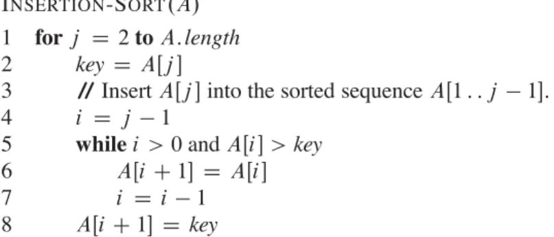
When the first two properties hold, the loop invariant is true before each iteration of the loop. Furthermore, this substring is sorted (trivially, of course), indicating that the loop invariant holds before the first iteration of the loop.
Analyzing algorithms
The worst-case running time of the algorithm gives us an upper bound on the running time for any input. We write that insertion sort has the worst possible running time‚.n2/(pronounced “theta ofn-squared”).
Designing algorithms
The divide-and-conquer approach
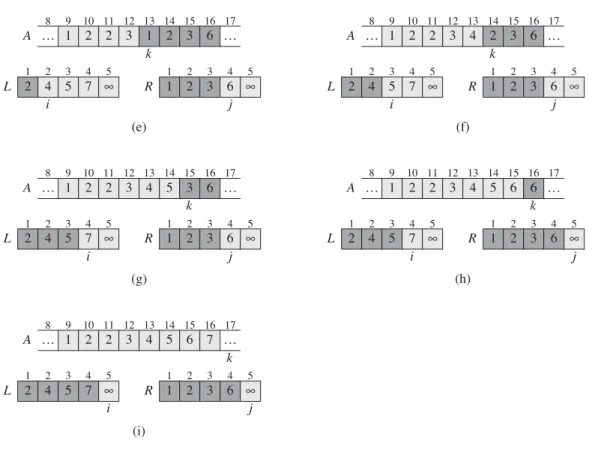
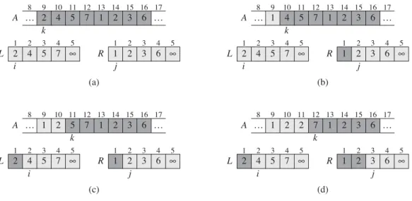
The heavily shaded positions in Contains values to be copied, and the heavily shaded positions in Earth contain values that have already been copied back to A. a)–(h) ArraysA,L, and R and their corresponding index, i, forward each loop repeat of rows 12–17. Initialization: Before the first iteration of the loop, we have Dp, so that the subsetAŒp : : k1 is empty.
Analyzing divide-and-conquer algorithms
A runtime iteration of a divide-and-conquer algorithm falls out of the three steps of the basic paradigm. Shell, which uses insertion sort on periodic subsequences of the input to produce a faster sorting algorithm.
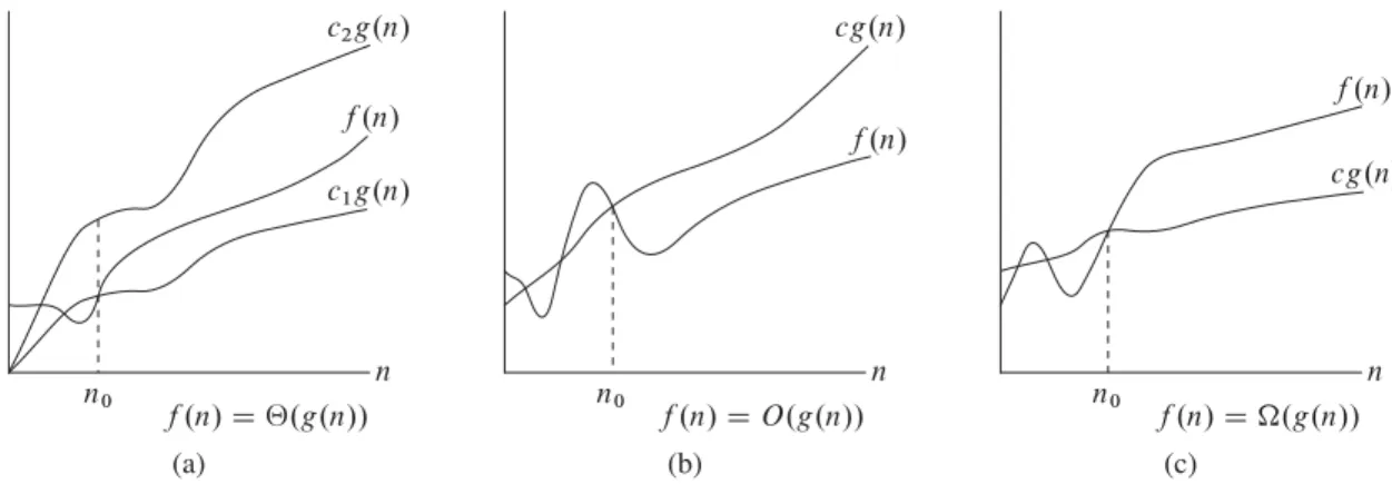
Asymptotic notation
In Chapter 2, we found that the worst-case execution time of insertion sort is T .n/D‚.n2/. Let's define what this note means. Thus, theO.n2/ bound on the worst-case execution time of the input order also applies to its execution time on each input. Equivalently, we are giving a lower bound for the best running time of an algorithm.
For example, in Chapter 2 we expressed the worst-case running time of merge sort as the iteration.
Standard notations and common functions
What happens to each direction of the "axis and only axis" in Theorem 3.1 if we substitute O0 for O but still use For each of the following functionsf .n/and constantsc, give as narrow a limit as possible onfc.n/. In Section 2.3.1, we saw how merge sort serves as an example of the divide-and-recover paradigm.
For example, in Section 2.3.2 we described the worst-case running time T .n/ of the MERGE-SORT procedure by the iteration T .n/D.
The maximum-subarray problem
Let's think about how we can solve the maximum substring problem using the divide-and-conquer technique. We can easily find a maximal subgroup that crosses the midpoint in linear time in the subgroup size AŒlow: :high. Apply both brute-force and recursive algorithms to the maximum underload problem on your computer.
Use the following ideas to develop a non-recursive, linear-time algorithm for the maximum subarray problem.

Strassen’s algorithm for matrix multiplication
Because each of the thrice-nested for loops executes exactly iterations, and each execution of line 7 takes a constant time, the SQUARE-MATRIX-COMPUBLIC procedure takes .n3/time. Each of these matrices contains n2=4 entries, so each of the four matrix additions takes n2/time. The right column only shows what these products are equal to in terms of the original submatrices created in step 1.
The notes at the end of this chapter discuss some of the practical aspects of Strassen's algorithm.
The substitution method for solving recurrences
Mathematical induction now requires us to show that our solution holds for the boundary conditions. Typically, we do this by showing that the boundary conditions are suitable as base cases for the inductive proof. For the iteration (4.19) we have to show that we can choose the constant c large enough so that the bound T .n/cnlgn also works for the boundary conditions.
Show that by making another inductive hypothesis we can overcome the difficulty with the constraint T .1/D1 for recurrence (4.19) without modifying the constraints for the inductive proof.
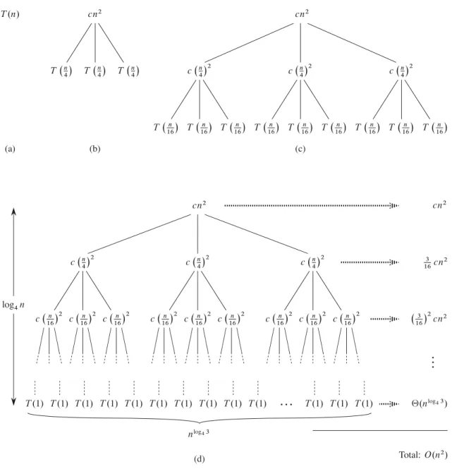
The recursion-tree method for solving recurrences
As a result, levels at the bottom of the recursion tree contribute less to the total cost. Use a recursion tree to determine a good asymptotic upper bound for the recurrence T .n/DT .n1/CT .n=2/Cn. Use a recursion tree to give an asymptotically tight solution to the recursion T .n/DT .na/CT .a/Ccn, where a1andc > 0 are constants.
Use a recursion tree to give an asymptotically tight solution to the iteration T .n/DT .˛ n/CT .1˛/n/Ccn, where ˛ is a constant in the range 0 < ˛ < 1 andc > 0 is also a constant.
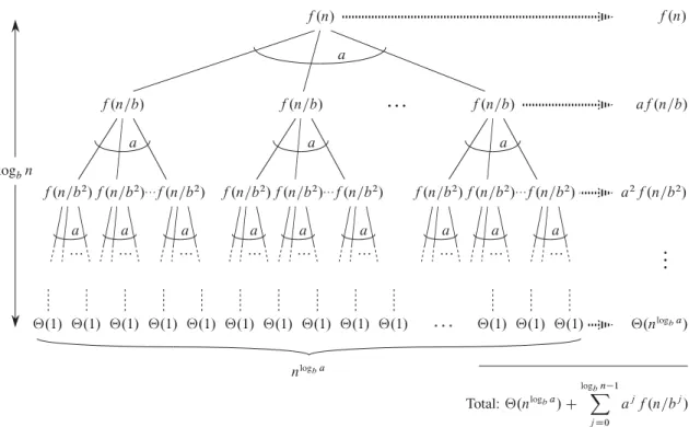
The master method for solving recurrences
The proof for exact powers
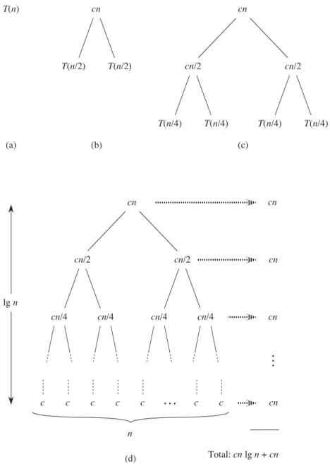
The third lemma combines the first two to prove a version of the main theorem for the case in which the exact power is b. Equation (4.21) can be obtained by summing the costs of the nodes at each depth in the tree as shown in the figure. The summation in equation (4.21) describes the cost of the division and union steps in the basic divide-and-conquer algorithm.
We can now prove a version of the main theorem for the case where there is an exact quench.
Floors and ceilings
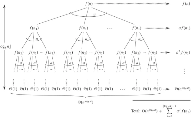
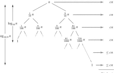
In other words, because of the limited precision of computer calculations on non-integers, larger errors accumulate in Strassen's algorithm than in SQUARE-MATRIX-MULTIPLY. The Akra-Bazzi method works for relapses of the form. k1 is an integer constant, and. While the master method does not apply to a repetition such as T .n/ D T .bn=3c/CT .b2n=3c/CO.n/, the Akra-Bazzi method does.
To solve the iteration (4.30), we first find the unique real number such as Pk. Such always exist.) The solution to the repetition is then T .n/D‚.
Algorithms
The hiring problem
To use probabilistic analysis, we need to know something about the distribution of inputs. Let's say the temp agency has n candidates and they send us a list of the candidates in advance. Instead of relying on a guess that the candidates will come to us in a random order, we have instead taken control of the process and enforced a random order.
When analyzing the running time of a random algorithm, we take the expectation of the running time over the distribution of values returned by the random number generator.
Indicator random variables
For example, indicator random variables allow us a simple way to arrive at the result of equation (C.37). Thus, compared to the method used in equation (C.37), indicator random variables greatly simplify the calculation. In particular, we let Xibe be an indicator random variable associated with the event in which the candidate is employed.
Use indicator random variables to solve the following problem, known as the hat check problem.
Randomized algorithms
- The birthday paradox
- Balls and bins
- Streaks
- The on-line hiring problem
The probability that at least two of the birthdays match is 1minus the probability that all the birthdays are different. We first prove that the expected length of the longest streak of heads is O.lgn/. We now prove a complementary lower bound: the expected length of the longest streak heads inncoin flips is.lgn/.
From these rough estimates alone, we can conclude that the expected length of the longest streak is‚.lgn/.
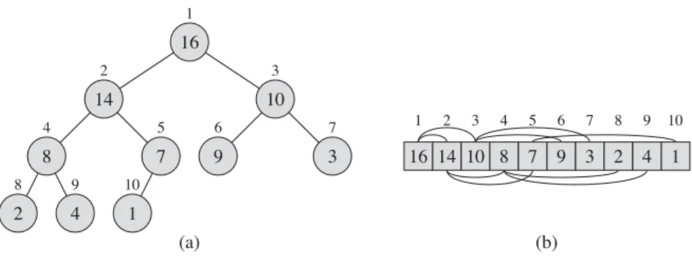
Heaps
In amax-heap, the max-heap property is that of every nodei other than the root. Thus, the largest element in a max-heap is stored at the root, and the subtree rooted at a node contains The MAX-HEAPIFY procedure, which runs iO.lgn/hour, is the key to maintaining the max-heap property.
The MAX-HOOP-INSERT, HEAP-EXTRACT-MAX, HEAP-INCREASE-KEY, and HEAP-MAXIMUM procedures, which run inO.lgn/time, allow the heap data structure to implement a priority queue.
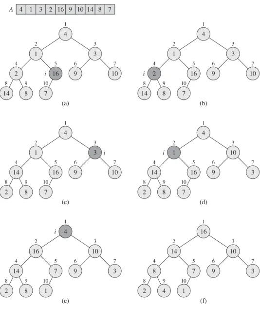
Maintaining the heap property
After replacing AŒ4 with AŒ9 as shown in (c), node4 is fixed and recursively calls MAX-HEAPIFY.A; 9/does not result in any further changes to the data structure. The running time of MAX-HEAPIFY on a subtree of size n rooted at a given node i is ‚.1/ the time to correct the relationships between the elements AŒi, AŒLEFT.i / and AŒRIGHT.i /, plus the time to run MAX-HEAPIFY on the subtree rooted in one of the node's children (assuming a recursive call occurs). What is the effect of calling MAX-HEAPIFY.A; i /when elementAŒi is greater than its children.
Write an efficient MAX-HEAPIFY that uses an iterative control construct (a loop) instead of recursion.

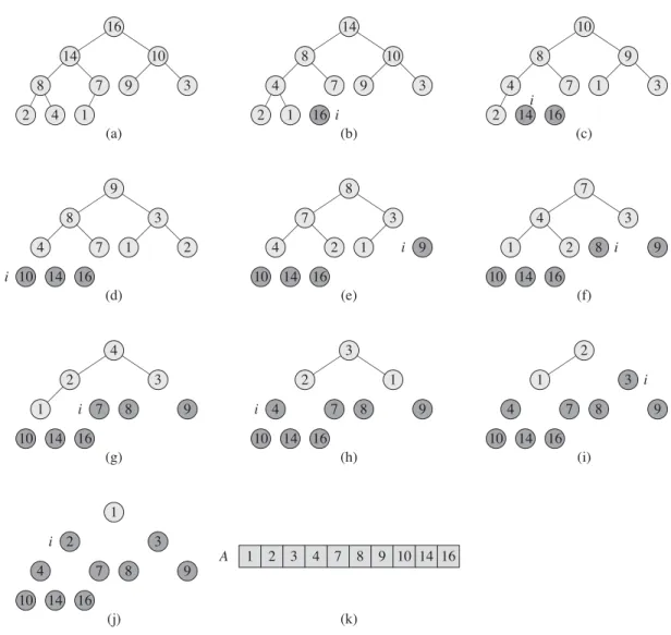
Building a heap
The BUILD-MAX-HEAP procedure loops through the remaining nodes in the tree and runs MAX-HEAPIFY on each one. We can calculate a simple upper bound on the runtime of BUILD-MAX-HEAP as follows. Each call to MAX-HEAPIFY costs O.lgn/time, and BUILD-MAX-HEAP makes O.n/ such calls.
Note that whenever MAX-HEAPIFY is called on a node, the two subtrees of that node are both max-heaps. f) Maximum platoon after completion of BUILD-MAX-HEAP.
The heapsort algorithm
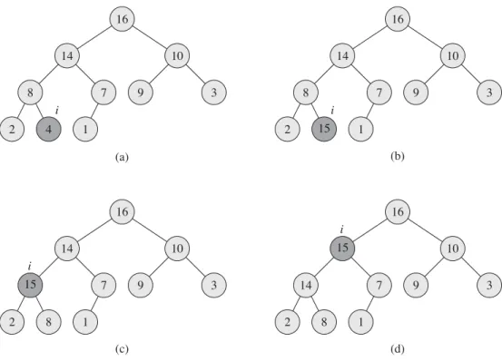
If we now discard node n from the heap - and we can do this by simply reducing A:heap-size - we notice that the children of the root remain max-heap, but the new root element might violate the max-heap property. The heapsort algorithm then repeats this process for the largest size1 heap up to the size2 heap. The figure shows the max-heap before the first iteration of the forloop lines 2–5 and after each iteration.
The HEAP SORT procedure takes time.log n/, since the call to BUILD-MAX-HEAP takes time O.n/ and each of the n 1 calls to MAX-HEAPIFY takes timeO.lgn/.
Priority queues
The procedure first expands the max-heap by adding a new leaf to the tree whose key is 1. It then calls HEAP-INCREASE-KEY to set the key of this new node to the correct value and preserve the max-heap property. You can assume that the subarray AŒ1 : : A:heap-size satisfies the max-heap property at the time of the HEAP-INCREASE-KEY call.
Give an implementation of HEAP-DELETE that runs in O.lgn/hour for an n-element max-heap.
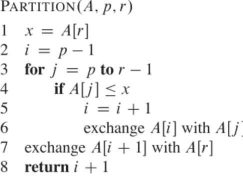
Description of quicksort
At the beginning of each iteration of the loop of lines 3-6, for any array indexk,. The unshaded elements have not yet been put into either of the first two partitions, and the final white element is pivotx.(a) The initial array and variable settings. Neither element has been placed in either of the first two partitions. (b) The value 2 is swapped with itself and put in the partition with smaller values. (c)–(d) The values 8 and 7 are added to the partition with larger values. .(e)The values 1 and 8 are swapped and the smaller partition grows. f)The values3and7 are swapped and the smaller partition grows.(g)–(h)The larger partition grows to include5and6 and the loop ends.(i)In lines 7–8, the pivot element is swapped so that it lies between the two partitions.
In fact, it satisfies a slightly stronger condition: after line 2 of QUICKSORT, AŒq is strictly less than each element of AŒqC1 : : r. Figure 7.3 The two cases for one iteration of procedure PARTITION. a)IfAŒj > x, the only action is to incrementrej, which keeps the loop invariant.(b)IfAŒj x, indexiis incremented, AŒi andAŒj are swapped, and thenj is incremented.
Performance of quicksort
Thus, if the partition is maximally unbalanced at each recursive level of the algorithm, the running time is ‚.n2/. By equally balancing both sides of the partition at each level of recursion, we obtain an asymptotically faster algorithm. Partitioning the subset of sizen1costsn1and produces a "good" partition: subsets of sizes.n1/=21and.n1/=2. b) A single level of a recursion tree that is very well balanced.
We will provide a rigorous analysis of the expected runtime of a randomized version of quicksort in section 7.4.2.
A randomized version of quicksort