[Katsuhiko Ogata] Modern Control Engineering

(1)

(2)

Modern Control Engineering

Fifth Edition

Katsuhiko Ogata

Prentice Hall

Boston Columbus Indianapolis New York San Francisco Upper Saddle River Amsterdam Cape Town Dubai London Madrid Milan Munich Paris Montreal Toronto

Delhi Mexico City Sao Paulo Sydney Hong Kong Seoul Singapore Taipei Tokyo

(3)

VP/Editorial Director, Engineering/Computer Science: Marcia J. Horton Assistant/Supervisor: Dolores Mars

Senior Editor: Andrew Gilfillan Associate Editor: Alice Dworkin Editorial Assistant: William Opaluch Director of Marketing: Margaret Waples Senior Marketing Manager: Tim Galligan Marketing Assistant: Mack Patterson Senior Managing Editor: Scott Disanno Art Editor: Greg Dulles

Senior Operations Supervisor: Alan Fischer Operations Specialist: Lisa McDowell Art Director: Kenny Beck

Cover Designer: Carole Anson Media Editor: Daniel Sandin

Credits and acknowledgments borrowed from other sources and reproduced, with permission, in this textbook appear on appropriate page within text.

MATLAB is a registered trademark of The Mathworks, Inc., 3 Apple Hill Drive, Natick MA 01760-2098.

Copyright © 2010, 2002, 1997, 1990, 1970 Pearson Education, Inc., publishing as Prentice Hall, One Lake Street, Upper Saddle River, New Jersey 07458. All rights reserved. Manufactured in the United States of America. This publication is protected by Copyright, and permission should be obtained from the publisher prior to any prohibited reproduction, storage in a retrieval system, or transmission in any form or by any means, electronic, mechanical, photocopying, recording, or likewise. To obtain permission(s) to use material from this work, please submit a written request to Pearson Education, Inc., Permissions Department, One Lake Street, Upper Saddle River, New Jersey 07458.

Many of the designations by manufacturers and seller to distinguish their products are claimed as trademarks. Where those designations appear in this book, and the publisher was aware of a trademark claim, the designations have been printed in initial caps or all caps.

Library of Congress Cataloging-in-Publication Data on File

10 9 8 7 6 5 4 3 2 1

ISBN 10: 0-13-615673-8 ISBN 13: 978-0-13-615673-4

(4)

C

iii

This page intentionally left blank

(10)

P

ix

Preface

This book introduces important concepts in the analysis and design of control systems.

Readers will find it to be a clear and understandable textbook for control system courses at colleges and universities. It is written for senior electrical, mechanical, aerospace, or chemical engineering students. The reader is expected to have fulfilled the following prerequisites: introductory courses on differential equations, Laplace transforms, vector- matrix analysis, circuit analysis, mechanics, and introductory thermodynamics.

The main revisions made in this edition are as follows:

• The use of MATLAB for obtaining responses of control systems to various inputs has been increased.

• The usefulness of the computational optimization approach with MATLAB has been demonstrated.

• New example problems have been added throughout the book.

• Materials in the previous edition that are of secondary importance have been deleted in order to provide space for more important subjects. Signal flow graphs were dropped from the book. A chapter on Laplace transform was deleted. Instead, Laplace transform tables, and partial-fraction expansion with MATLAB are presented in Appendix A and Appendix B, respectively.

• A short summary of vector-matrix analysis is presented in Appendix C; this will help the reader to find the inverses of n x n matrices that may be involved in the analysis and design of control systems.

This edition of Modern Control Engineeringis organized into ten chapters.The outline of this book is as follows: Chapter 1 presents an introduction to control systems. Chapter 2

(11)

deals with mathematical modeling of control systems. A linearization technique for nonlinear mathematical models is presented in this chapter. Chapter 3 derives mathematical models of mechanical systems and electrical systems. Chapter 4 discusses mathematical modeling of fluid systems (such as liquid-level systems, pneumatic systems, and hydraulic systems) and thermal systems.

Chapter 5 treats transient response and steady-state analyses of control systems.

MATLAB is used extensively for obtaining transient response curves. Routh’s stability criterion is presented for stability analysis of control systems. Hurwitz stability criterion is also presented.

Chapter 6 discusses the root-locus analysis and design of control systems, including positive feedback systems and conditionally stable systems Plotting root loci with MAT- LAB is discussed in detail. Design of lead, lag, and lag-lead compensators with the root- locus method is included.

Chapter 7 treats the frequency-response analysis and design of control systems. The Nyquist stability criterion is presented in an easily understandable manner. The Bode diagram approach to the design of lead, lag, and lag-lead compensators is discussed.

Chapter 8 deals with basic and modified PID controllers. Computational approaches for obtaining optimal parameter values for PID controllers are discussed in detail, par- ticularly with respect to satisfying requirements for step-response characteristics.

Chapter 9 treats basic analyses of control systems in state space. Concepts of con- trollability and observability are discussed in detail.

Chapter 10 deals with control systems design in state space. The discussions include pole placement, state observers, and quadratic optimal control. An introductory discussion of robust control systems is presented at the end of Chapter 10.

The book has been arranged toward facilitating the student’s gradual understanding of control theory. Highly mathematical arguments are carefully avoided in the presen- tation of the materials. Statement proofs are provided whenever they contribute to the understanding of the subject matter presented.

Special effort has been made to provide example problems at strategic points so that the reader will have a clear understanding of the subject matter discussed. In addition, a number of solved problems (A-problems) are provided at the end of each chapter, except Chapter 1. The reader is encouraged to study all such solved problems carefully;

this will allow the reader to obtain a deeper understanding of the topics discussed. In addition, many problems (without solutions) are provided at the end of each chapter, except Chapter 1. The unsolved problems (B-problems) may be used as homework or quiz problems.

If this book is used as a text for a semester course (with 56 or so lecture hours), a good portion of the material may be covered by skipping certain subjects. Because of the abundance of example problems and solved problems (A-problems) that might answer many possible questions that the reader might have, this book can also serve as a self- study book for practicing engineers who wish to study basic control theories.

I would like to thank the following reviewers for this edition of the book: Mark Camp- bell, Cornell University; Henry Sodano, Arizona State University; and Atul G. Kelkar, Iowa State University. Finally, I wish to offer my deep appreciation to Ms.Alice Dworkin, Associate Editor, Mr. Scott Disanno, Senior Managing Editor, and all the people involved in this publishing project, for the speedy yet superb production of this book.

Katsuhiko Ogata

(12)

1

Introduction to Control Systems

1–1 INTRODUCTION

Control theories commonly used today are classical control theory (also called con- ventional control theory), modern control theory, and robust control theory. This book presents comprehensive treatments of the analysis and design of control systems based on the classical control theory and modern control theory. A brief introduction of robust control theory is included in Chapter 10.

Automatic control is essential in any field of engineering and science. Automatic control is an important and integral part of space-vehicle systems, robotic systems, modern manufacturing systems, and any industrial operations involving control of temperature, pressure, humidity, flow, etc. It is desirable that most engineers and scientists are familiar with theory and practice of automatic control.

This book is intended to be a text book on control systems at the senior level at a college or university. All necessary background materials are included in the book. Math- ematical background materials related to Laplace transforms and vector-matrix analysis are presented separately in appendixes.

Brief Review of Historical Developments of Control Theories and Practices.

The first significant work in automatic control was James Watt’s centrifugal gover- nor for the speed control of a steam engine in the eighteenth century. Other significant works in the early stages of development of control theory were due to

1

(13)

Minorsky, Hazen, and Nyquist, among many others. In 1922, Minorsky worked on automatic controllers for steering ships and showed how stability could be determined from the differential equations describing the system. In 1932, Nyquist developed a relatively simple procedure for determining the stability of closed-loop systems on the basis of open-loop response to steady-state sinusoidal inputs. In 1934, Hazen, who introduced the term servomechanisms for position control systems, discussed the design of relay servomechanisms capable of closely following a changing input.

During the decade of the 1940s, frequency-response methods (especially the Bode diagram methods due to Bode) made it possible for engineers to design linear closed- loop control systems that satisfied performance requirements. Many industrial control systems in 1940s and 1950s used PID controllers to control pressure, temperature, etc.

In the early 1940s Ziegler and Nichols suggested rules for tuning PID controllers, called Ziegler–Nichols tuning rules. From the end of the 1940s to the 1950s, the root-locus method due to Evans was fully developed.

The frequency-response and root-locus methods, which are the core of classical control theory, lead to systems that are stable and satisfy a set of more or less arbitrary performance requirements. Such systems are, in general, acceptable but not optimal in any meaningful sense. Since the late 1950s, the emphasis in control design problems has been shifted from the design of one of many systems that work to the design of one optimal system in some meaningful sense.

As modern plants with many inputs and outputs become more and more complex, the description of a modern control system requires a large number of equations. Clas- sical control theory, which deals only with single-input, single-output systems, becomes powerless for multiple-input, multiple-output systems. Since about 1960, because the availability of digital computers made possible time-domain analysis of complex systems, modern control theory, based on time-domain analysis and synthesis using state variables, has been developed to cope with the increased complexity of modern plants and the stringent requirements on accuracy, weight, and cost in military, space, and industrial applications.

During the years from 1960 to 1980, optimal control of both deterministic and sto- chastic systems, as well as adaptive and learning control of complex systems, were fully investigated. From 1980s to 1990s, developments in modern control theory were cen- tered around robust control and associated topics.

Modern control theory is based on time-domain analysis of differential equation systems. Modern control theory made the design of control systems simpler because the theory is based on a model of an actual control system. However, the system’s stability is sensitive to the error between the actual system and its model. This means that when the designed controller based on a model is applied to the actual system, the system may not be stable. To avoid this situation, we design the control system by first setting up the range of possible errors and then designing the controller in such a way that, if the error of the system stays within the assumed range, the designed control system will stay stable. The design method based on this principle is called robust control theory. This theory incorporates both the frequency- response approach and the time-domain approach. The theory is mathematically very complex.

(14)

Section 1–1 / Introduction 3 Because this theory requires mathematical background at the graduate level, inclu- sion of robust control theory in this book is limited to introductory aspects only. The reader interested in details of robust control theory should take a graduate-level control course at an established college or university.

Definitions. Before we can discuss control systems, some basic terminologies must be defined.

Controlled Variable and Control Signal or Manipulated Variable. The controlled variable is the quantity or condition that is measured and controlled. Thecontrol signal ormanipulatedvariable is the quantity or condition that is varied by the controller so as to affect the value of the controlled variable. Normally, the controlled variable is the output of the system.Controlmeans measuring the value of the controlled variable of the system and applying the control signal to the system to correct or limit deviation of the measured value from a desired value.

In studying control engineering, we need to define additional terms that are necessary to describe control systems.

Plants. A plant may be a piece of equipment, perhaps just a set of machine parts functioning together, the purpose of which is to perform a particular operation. In this book, we shall call any physical object to be controlled (such as a mechanical device, a heating furnace, a chemical reactor, or a spacecraft) a plant.

Processes. The Merriam–Webster Dictionarydefines a process to be a natural, progressively continuing operation or development marked by a series of gradual changes that succeed one another in a relatively fixed way and lead toward a particular result or end; or an artificial or voluntary, progressively continuing operation that consists of a series of controlled actions or movements systematically directed toward a particular result or end. In this book we shall call any operation to be controlled a process.Examples are chemical, economic, and biological processes.

Systems. A system is a combination of components that act together and perform a certain objective. A system need not be physical. The concept of the system can be applied to abstract, dynamic phenomena such as those encountered in economics. The word system should, therefore, be interpreted to imply physical, biological, economic, and the like, systems.

Disturbances. A disturbance is a signal that tends to adversely affect the value of the output of a system. If a disturbance is generated within the system, it is called internal, while an external disturbance is generated outside the system and is an input.

Feedback Control. Feedback control refers to an operation that, in the presence of disturbances, tends to reduce the difference between the output of a system and some reference input and does so on the basis of this difference. Here only unpredictable disturbances are so specified, since predictable or known disturbances can always be com- pensated for within the system.

(15)

1–2 EXAMPLES OF CONTROL SYSTEMS

In this section we shall present a few examples of control systems.

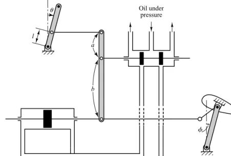
Speed Control System. The basic principle of a Watt’s speed governor for an engine is illustrated in the schematic diagram of Figure 1–1. The amount of fuel admitted to the engine is adjusted according to the difference between the desired and the actual engine speeds.

The sequence of actions may be stated as follows: The speed governor is adjusted such that, at the desired speed, no pressured oil will flow into either side of the power cylinder. If the actual speed drops below the desired value due to disturbance, then the decrease in the centrifugal force of the speed governor causes the control valve to move downward, supplying more fuel, and the speed of the engine increases until the desired value is reached. On the other hand, if the speed of the engine increases above the desired value, then the increase in the centrifugal force of the governor causes the control valve to move upward. This decreases the supply of fuel, and the speed of the engine decreases until the desired value is reached.

In this speed control system, the plant (controlled system) is the engine and the controlled variable is the speed of the engine. The difference between the desired speed and the actual speed is the error signal. The control signal (the amount of fuel) to be applied to the plant (engine) is the actuating signal. The external input to dis- turb the controlled variable is the disturbance. An unexpected change in the load is a disturbance.

Temperature Control System. Figure 1–2 shows a schematic diagram of temperature control of an electric furnace. The temperature in the electric furnace is measured by a thermometer, which is an analog device. The analog temperature is converted

Oil under pressure

Power cylinder

Close Open Pilot

valve

Control valve Fuel

Engine Load

Figure 1–1 Speed control system.

(16)

Section 1–2 / Examples of Control Systems 5 Thermometer

Heater

Interface

Controller

Interface Amplifier

A/D converter

Programmed input Electric

furnace

Relay Figure 1–2

Temperature control system.

to a digital temperature by an A/D converter. The digital temperature is fed to a controller through an interface. This digital temperature is compared with the programmed input temperature, and if there is any discrepancy (error), the controller sends out a signal to the heater, through an interface, amplifier, and relay, to bring the furnace temperature to a desired value.

Business Systems. A business system may consist of many groups. Each task assigned to a group will represent a dynamic element of the system. Feedback methods of reporting the accomplishments of each group must be established in such a system for proper operation. The cross-coupling between functional groups must be made a mini- mum in order to reduce undesirable delay times in the system. The smaller this cross- coupling, the smoother the flow of work signals and materials will be.

A business system is a closed-loop system. A good design will reduce the manageri- al control required. Note that disturbances in this system are the lack of personnel or materials, interruption of communication, human errors, and the like.

The establishment of a well-founded estimating system based on statistics is manda- tory to proper management. It is a well-known fact that the performance of such a system can be improved by the use of lead time, or anticipation.

To apply control theory to improve the performance of such a system, we must represent the dynamic characteristic of the component groups of the system by a relatively simple set of equations.

Although it is certainly a difficult problem to derive mathematical representations of the component groups, the application of optimization techniques to business systems significantly improves the performance of the business system.

Consider, as an example, an engineering organizational system that is composed of major groups such as management, research and development, preliminary design, experiments, product design and drafting, fabrication and assembling, and tesing. These groups are interconnected to make up the whole operation.

Such a system may be analyzed by reducing it to the most elementary set of components necessary that can provide the analytical detail required and by representing the dynamic characteristics of each component by a set of simple equations. (The dynamic performance of such a system may be determined from the relation between progres- sive accomplishment and time.)

(17)

Required product

Management

Research and development

Preliminary

design Experiments

Product design and

drafting

Fabrication and assembling

Testing

Product

Figure 1–3

Block diagram of an engineering organizational system.

A functional block diagram may be drawn by using blocks to represent the functional activities and interconnecting signal lines to represent the information or product output of the system operation. Figure 1–3 is a possible block diagram for this system.

Robust Control System. The first step in the design of a control system is to obtain a mathematical model of the plant or control object. In reality, any model of a plant we want to control will include an error in the modeling process. That is, the actual plant differs from the model to be used in the design of the control system.

To ensure the controller designed based on a model will work satisfactorily when this controller is used with the actual plant, one reasonable approach is to assume from the start that there is an uncertainty or error between the actual plant and its mathematical model and include such uncertainty or error in the design process of the control system. The control system designed based on this approach is called a robust control system.

Suppose that the actual plant we want to control is (s)and the mathematical model of the actual plant is G(s), that is,

(s)=actual plant model that has uncertainty ¢(s)

G(s)=nominal plant model to be used for designing the control system (s)andG(s)may be related by a multiplicative factor such as

or an additive factor

or in other forms.

Since the exact description of the uncertainty or error ¢(s)is unknown, we use an estimate of ¢(s)and use this estimate,W(s), in the design of the controller.W(s)is a scalar transfer function such that

where is the maximum value of for and is called the H infinity norm of W(s).

0v q

冟W(jv)冟冟冟W(s)冟冟q

冟冟¢(s)冟冟q 6 冟冟W(s)冟冟q = max

0vq冟W(jv)冟 G苲(s) = G(s) + ¢(s)

G苲(s) = G(s)[1 +¢(s)]

G苲

(18)

Section 1–3 / Closed-Loop Control versus Open-Loop Control 7 Using the small gain theorem, the design procedure here boils down to the determination of the controller K(s)such that the inequality

is satisfied, where G(s)is the transfer function of the model used in the design process, K(s)is the transfer function of the controller, and W(s)is the chosen transfer function to approximate ¢(s). In most practical cases, we must satisfy more than one such inequality that involves G(s),K(s), and W(s)’s. For example, to guarantee robust stability and robust performance we may require two inequalities, such as

for robust stability

for robust performance

be satisfied. (These inequalities are derived in Section 10–9.) There are many different such inequalities that need to be satisfied in many different robust control systems.

(Robust stability means that the controller K(s)guarantees internal stability of all systems that belong to a group of systems that include the system with the actual plant.

Robust performance means the specified performance is satisfied in all systems that belong to the group.) In this book all the plants of control systems we discuss are assumed to be known precisely, except the plants we discuss in Section 10–9 where an introductory aspect of robust control theory is presented.

1–3 CLOSED-LOOP CONTROL VERSUS OPEN-LOOP CONTROL

Feedback Control Systems. A system that maintains a prescribed relationship between the output and the reference input by comparing them and using the difference as a means of control is called a feedback control system.An example would be a room- temperature control system. By measuring the actual room temperature and comparing it with the reference temperature (desired temperature), the thermostat turns the heating or cooling equipment on or off in such a way as to ensure that the room temperature remains at a comfortable level regardless of outside conditions.

Feedback control systems are not limited to engineering but can be found in various nonengineering fields as well. The human body, for instance, is a highly advanced feedback control system. Both body temperature and blood pressure are kept constant by means of physiological feedback. In fact, feedback performs a vital function: It makes the human body relatively insensitive to external disturbances, thus enabling it to function properly in a changing environment.

ß Ws(s)

1 + K(s)G(s)ß

q

6 1 ßW_m(s)K(s)G(s)

1 + K(s)G(s) ß

q

6 1

ß W(s)

1 + K(s)G(s)ß

q

6 1

(19)

Closed-Loop Control Systems. Feedback control systems are often referred to asclosed-loop controlsystems. In practice, the terms feedback control and closed-loop control are used interchangeably. In a closed-loop control system the actuating error signal, which is the difference between the input signal and the feedback signal (which may be the output signal itself or a function of the output signal and its derivatives and/or integrals), is fed to the controller so as to reduce the error and bring the output of the system to a desired value. The term closed-loop control always implies the use of feedback control action in order to reduce system error.

Open-Loop Control Systems. Those systems in which the output has no effect on the control action are called open-loop control systems.In other words, in an open- loop control system the output is neither measured nor fed back for comparison with the input. One practical example is a washing machine. Soaking, washing, and rinsing in the washer operate on a time basis. The machine does not measure the output signal, that is, the cleanliness of the clothes.

In any open-loop control system the output is not compared with the reference input.

Thus, to each reference input there corresponds a fixed operating condition; as a result, the accuracy of the system depends on calibration. In the presence of disturbances, an open-loop control system will not perform the desired task. Open-loop control can be used, in practice, only if the relationship between the input and output is known and if there are neither internal nor external disturbances. Clearly, such systems are not feedback control systems. Note that any control system that operates on a time basis is open loop. For instance, traffic control by means of signals operated on a time basis is another example of open-loop control.

Closed-Loop versus Open-Loop Control Systems. An advantage of the closed- loop control system is the fact that the use of feedback makes the system response relatively insensitive to external disturbances and internal variations in system parameters.

It is thus possible to use relatively inaccurate and inexpensive components to obtain the accurate control of a given plant, whereas doing so is impossible in the open-loop case.

From the point of view of stability, the open-loop control system is easier to build because system stability is not a major problem. On the other hand, stability is a major problem in the closed-loop control system, which may tend to overcorrect errors and thereby can cause oscillations of constant or changing amplitude.

It should be emphasized that for systems in which the inputs are known ahead of time and in which there are no disturbances it is advisable to use open-loop control.

Closed-loop control systems have advantages only when unpredictable disturbances and/or unpredictable variations in system components are present. Note that the output power rating partially determines the cost, weight, and size of a control system.

The number of components used in a closed-loop control system is more than that for a corresponding open-loop control system. Thus, the closed-loop control system is generally higher in cost and power. To decrease the required power of a system, open- loop control may be used where applicable. A proper combination of open-loop and closed-loop controls is usually less expensive and will give satisfactory overall system performance.

Most analyses and designs of control systems presented in this book are concerned with closed-loop control systems. Under certain circumstances (such as where no disturbances exist or the output is hard to measure) open-loop control systems may be

(20)

desired. Therefore, it is worthwhile to summarize the advantages and disadvantages of using open-loop control systems.

The major advantages of open-loop control systems are as follows:

1. Simple construction and ease of maintenance.

2. Less expensive than a corresponding closed-loop system.

3. There is no stability problem.

4. Convenient when output is hard to measure or measuring the output precisely is economically not feasible. (For example, in the washer system, it would be quite expensive to provide a device to measure the quality of the washer’s output, cleanliness of the clothes.)

The major disadvantages of open-loop control systems are as follows:

1. Disturbances and changes in calibration cause errors, and the output may be different from what is desired.

2. To maintain the required quality in the output, recalibration is necessary from time to time.

1–4 DESIGN AND COMPENSATION OF CONTROL SYSTEMS

This book discusses basic aspects of the design and compensation of control systems.

Compensation is the modification of the system dynamics to satisfy the given specifications. The approaches to control system design and compensation used in this book are the root-locus approach, frequency-response approach, and the state-space approach. Such control systems design and compensation will be presented in Chapters 6, 7, 9 and 10. The PID-based compensational approach to control systems design is given in Chapter 8.

In the actual design of a control system, whether to use an electronic, pneumatic, or hydraulic compensator is a matter that must be decided partially based on the nature of the controlled plant. For example, if the controlled plant involves flammable fluid, then we have to choose pneumatic components (both a compensator and an actuator) to avoid the possibility of sparks. If, however, no fire hazard exists, then electronic compensators are most commonly used. (In fact, we often transform nonelectrical signals into electrical signals because of the simplicity of transmission, increased accuracy, increased reliability, ease of compensation, and the like.)

Performance Specifications. Control systems are designed to perform specific tasks. The requirements imposed on the control system are usually spelled out as performance specifications. The specifications may be given in terms of transient response requirements (such as the maximum overshoot and settling time in step response) and of steady-state requirements (such as steady-state error in following ramp input) or may be given in frequency-response terms. The specifications of a control system must be given before the design process begins.

For routine design problems, the performance specifications (which relate to accuracy, relative stability, and speed of response) may be given in terms of precise numerical values. In other cases they may be given partially in terms of precise numerical values and

Section 1–4 / Design and Compensation of Control Systems 9

(21)

partially in terms of qualitative statements. In the latter case the specifications may have to be modified during the course of design, since the given specifications may never be satisfied (because of conflicting requirements) or may lead to a very expensive system.

Generally, the performance specifications should not be more stringent than necessary to perform the given task. If the accuracy at steady-state operation is of prime importance in a given control system, then we should not require unnecessarily rigid performance specifications on the transient response, since such specifications will require expensive components. Remember that the most important part of control system design is to state the performance specifications precisely so that they will yield an optimal control system for the given purpose.

System Compensation. Setting the gain is the first step in adjusting the system for satisfactory performance. In many practical cases, however, the adjustment of the gain alone may not provide sufficient alteration of the system behavior to meet the given specifications. As is frequently the case, increasing the gain value will improve the steady-state behavior but will result in poor stability or even instability. It is then necessary to redesign the system (by modifying the structure or by incorporating additional devices or components) to alter the overall behavior so that the system will behave as desired. Such a redesign or addition of a suitable device is called compensa- tion.A device inserted into the system for the purpose of satisfying the specifications is called a compensator.The compensator compensates for deficient performance of the original system.

Design Procedures. In the process of designing a control system, we set up a mathematical model of the control system and adjust the parameters of a compensator.

The most time-consuming part of the work is the checking of the system performance by analysis with each adjustment of the parameters. The designer should use MATLAB or other available computer package to avoid much of the numerical drudgery necessary for this checking.

Once a satisfactory mathematical model has been obtained, the designer must con- struct a prototype and test the open-loop system. If absolute stability of the closed loop is assured, the designer closes the loop and tests the performance of the resulting closed- loop system. Because of the neglected loading effects among the components, nonlinearities, distributed parameters, and so on, which were not taken into consideration in the original design work, the actual performance of the prototype system will probably differ from the theoretical predictions. Thus the first design may not satisfy all the requirements on performance. The designer must adjust system parameters and make changes in the prototype until the system meets the specificications. In doing this, he or she must analyze each trial, and the results of the analysis must be incorporated into the next trial. The designer must see that the final system meets the performance apec- ifications and, at the same time, is reliable and economical.

1–5 OUTLINE OF THE BOOK

This text is organized into 10 chapters. The outline of each chapter may be summarized as follows:

Chapter 1 presents an introduction to this book.

(22)

Chapter 2 deals with mathematical modeling of control systems that are described by linear differential equations. Specifically, transfer function expressions of differential equation systems are derived. Also, state-space expressions of differential equation systems are derived. MATLAB is used to transform mathematical models from transfer functions to state-space equations and vice versa. This book treats linear systems in detail. If the mathematical model of any system is nonlinear, it needs to be linearized before applying theories presented in this book. A technique to linearize nonlinear mathematical models is presented in this chapter.

Chapter 3 derives mathematical models of various mechanical and electrical systems that appear frequently in control systems.

Chapter 4 discusses various fluid systems and thermal systems, that appear in control systems. Fluid systems here include liquid-level systems, pneumatic systems, and hydraulic systems. Thermal systems such as temperature control systems are also discussed here.

Control engineers must be familiar with all of these systems discussed in this chapter.

Chapter 5 presents transient and steady-state response analyses of control systems defined in terms of transfer functions. MATLAB approach to obtain transient and steady-state response analyses is presented in detail. MATLAB approach to obtain three-dimensional plots is also presented. Stability analysis based on Routh’s stability criterion is included in this chapter and the Hurwitz stability criterion is briefly discussed.

Chapter 6 treats the root-locus method of analysis and design of control systems. It is a graphical method for determining the locations of all closed-loop poles from the knowledge of the locations of the open-loop poles and zeros of a closed-loop system as a parameter (usually the gain) is varied from zero to infinity. This method was developed by W. R. Evans around 1950. These days MATLAB can produce root-locus plots easily and quickly. This chapter presents both a manual approach and a MATLAB approach to generate root-locus plots. Details of the design of control systems using lead compensators, lag compensators, are lag–lead compensators are presented in this chapter.

Chapter 7 presents the frequency-response method of analysis and design of control systems. This is the oldest method of control systems analysis and design and was developed during 1940–1950 by Nyquist, Bode, Nichols, Hazen, among others. This chapter presents details of the frequency-response approach to control systems design using lead compensation technique, lag compensation technique, and lag–lead compensation technique. The frequency-response method was the most frequently used analysis and design method until the state-space method became popular. However, since H-infinity control for designing robust control systems has become popular, frequency response is gaining popularity again.

Chapter 8 discusses PID controllers and modified ones such as multidegrees-of- freedom PID controllers. The PID controller has three parameters; proportional gain, integral gain, and derivative gain. In industrial control systems more than half of the controllers used have been PID controllers. The performance of PID controllers depends on the relative magnitudes of those three parameters. Determination of the relative magnitudes of the three parameters is called tuning of PID controllers.

Ziegler and Nichols proposed so-called “Ziegler–Nichols tuning rules” as early as 1942. Since then numerous tuning rules have been proposed. These days manufacturers of PID controllers have their own tuning rules. In this chapter we present a computer optimization approach using MATLAB to determine the three parameters to satisfy

Section 1–5 / Outline of the Book 11

(23)

given transient response characteristics.The approach can be expanded to determine the three parameters to satisfy any specific given characteristics.

Chapter 9 presents basic analysis of state-space equations. Concepts of controllabil- ity and observability, most important concepts in modern control theory, due to Kalman are discussed in full. In this chapter, solutions of state-space equations are derived in detail.

Chapter 10 discusses state-space designs of control systems. This chapter first deals with pole placement problems and state observers. In control engineering, it is frequently desirable to set up a meaningful performance index and try to minimize it (or maximize it, as the case may be). If the performance index selected has a clear physical meaning, then this approach is quite useful to determine the optimal control variable. This chapter discusses the quadratic optimal regulator problem where we use a performance index which is an integral of a quadratic function of the state variables and the control variable. The integral is performed from t=0tot= . This chapter concludes with a brief discussion of robust control systems.

q

(24)

2

13

Mathematical Modeling of Control Systems

2–1 INTRODUCTION

In studying control systems the reader must be able to model dynamic systems in mathematical terms and analyze their dynamic characteristics. A mathematical model of a dynamic system is defined as a set of equations that represents the dynamics of the system accurately, or at least fairly well. Note that a mathematical model is not unique to a given system. A system may be represented in many different ways and, therefore, may have many mathematical models, depending on one’s perspective.

The dynamics of many systems, whether they are mechanical, electrical, thermal, economic, biological, and so on, may be described in terms of differential equations.

Such differential equations may be obtained by using physical laws governing a particular system—for example, Newton’s laws for mechanical systems and Kirchhoff’s laws for electrical systems. We must always keep in mind that deriving reasonable mathematical models is the most important part of the entire analysis of control systems.

Throughout this book we assume that the principle of causality applies to the systems considered. This means that the current output of the system (the output at time t=0) depends on the past input (the input for t<0) but does not depend on the future input (the input for t>0).

Mathematical Models. Mathematical models may assume many different forms.

Depending on the particular system and the particular circumstances, one mathematical model may be better suited than other models. For example, in optimal control problems, it is advantageous to use state-space representations. On the other hand, for the

(25)

transient-response or frequency-response analysis of single-input, single-output, linear, time-invariant systems, the transfer-function representation may be more convenient than any other. Once a mathematical model of a system is obtained, various analytical and computer tools can be used for analysis and synthesis purposes.

Simplicity Versus Accuracy. In obtaining a mathematical model, we must make a compromise between the simplicity of the model and the accuracy of the results of the analysis. In deriving a reasonably simplified mathematical model, we frequently find it necessary to ignore certain inherent physical properties of the system. In particular, if a linear lumped-parameter mathematical model (that is, one employing ordinary differential equations) is desired, it is always necessary to ignore certain nonlinearities and distributed parameters that may be present in the physical system. If the effects that these ignored properties have on the response are small, good agreement will be obtained between the results of the analysis of a mathematical model and the results of the experimental study of the physical system.

In general, in solving a new problem, it is desirable to build a simplified model so that we can get a general feeling for the solution. A more complete mathematical model may then be built and used for a more accurate analysis.

We must be well aware that a linear lumped-parameter model, which may be valid in low-frequency operations, may not be valid at sufficiently high frequencies, since the neglected property of distributed parameters may become an important factor in the dynamic behavior of the system. For example, the mass of a spring may be neglected in low- frequency operations, but it becomes an important property of the system at high frequencies. (For the case where a mathematical model involves considerable errors, robust control theory may be applied. Robust control theory is presented in Chapter 10.)

Linear Systems. A system is called linear if the principle of superposition applies. The principle of superposition states that the response produced by the simultaneous application of two different forcing functions is the sum of the two individual responses. Hence, for the linear system, the response to several inputs can be calculated by treating one input at a time and adding the results. It is this principle that allows one to build up complicated solutions to the linear differential equation from simple solutions.

In an experimental investigation of a dynamic system, if cause and effect are proportional, thus implying that the principle of superposition holds, then the system can be considered linear.

Linear Time-Invariant Systems and Linear Time-Varying Systems. A differential equation is linear if the coefficients are constants or functions only of the independent variable. Dynamic systems that are composed of linear time-invariant lumped-parameter components may be described by linear time-invariant differential equations—that is, constant-coefficient differential equations. Such systems are called linear time-invariant (or linear constant-coefficient) systems. Systems that are represented by differential equations whose coefficients are functions of time are called linear time-varyingsystems. An example of a time-varying control system is a spacecraft control system. (The mass of a spacecraft changes due to fuel consumption.)

(26)

Section 2–2 / Transfer Function and Impulse-Response Function 15 Outline of the Chapter. Section 2–1 has presented an introduction to the mathematical modeling of dynamic systems. Section 2–2 presents the transfer function and impulse-response function. Section 2–3 introduces automatic control systems and Sec- tion 2–4 discusses concepts of modeling in state space. Section 2–5 presents state-space representation of dynamic systems. Section 2–6 discusses transformation of mathematical models with MATLAB. Finally, Section 2–7 discusses linearization of nonlinear mathematical models.

2–2 TRANSFER FUNCTION AND IMPULSE- RESPONSE FUNCTION

In control theory, functions called transfer functions are commonly used to character- ize the input-output relationships of components or systems that can be described by linear, time-invariant, differential equations. We begin by defining the transfer function and follow with a derivation of the transfer function of a differential equation system.

Then we discuss the impulse-response function.

Transfer Function. The transfer functionof a linear, time-invariant, differential equation system is defined as the ratio of the Laplace transform of the output (response function) to the Laplace transform of the input (driving function) under the assumption that all initial conditions are zero.

Consider the linear time-invariant system defined by the following differential equation:

whereyis the output of the system and xis the input. The transfer function of this system is the ratio of the Laplace transformed output to the Laplace transformed input when all initial conditions are zero, or

By using the concept of transfer function, it is possible to represent system dynamics by algebraic equations in s. If the highest power of sin the denominator of the transfer function is equal to n, the system is called an nth-order system.

Comments on Transfer Function. The applicability of the concept of the transfer function is limited to linear, time-invariant, differential equation systems. The transfer function approach, however, is extensively used in the analysis and design of such systems. In what follows, we shall list important comments concerning the transfer function. (Note that a system referred to in the list is one described by a linear, time-invariant, differential equation.)

= Y(s)

X(s) = b₀s^m + b₁s^m^-¹ + p + b_m_-₁s + b_m a₀sⁿ + a₁sⁿ^-¹ + p + a_n_-₁s + a_n Transfer function = G(s) = l[output]

l[input] 2

zero initial conditions

=b₀x

(m)

+ b₁x

(m-1)

+ p + b_m_-₁x#

+ b_mx

⁽ⁿ^m)

a₀y

(n)

+ a₁y

(n-1)

+ p + a_n_-₁y# + a_ny

(27)

1. The transfer function of a system is a mathematical model in that it is an opera- tional method of expressing the differential equation that relates the output variable to the input variable.

2. The transfer function is a property of a system itself, independent of the magnitude and nature of the input or driving function.

3. The transfer function includes the units necessary to relate the input to the output;

however, it does not provide any information concerning the physical structure of the system. (The transfer functions of many physically different systems can be identical.)

4. If the transfer function of a system is known, the output or response can be stud- ied for various forms of inputs with a view toward understanding the nature of the system.

5. If the transfer function of a system is unknown, it may be established experimen- tally by introducing known inputs and studying the output of the system. Once established, a transfer function gives a full description of the dynamic characteristics of the system, as distinct from its physical description.

Convolution Integral. For a linear, time-invariant system the transfer function G(s)is

whereX(s)is the Laplace transform of the input to the system and Y(s)is the Laplace transform of the output of the system, where we assume that all initial conditions involved are zero. It follows that the output Y(s)can be written as the product of G(s)and X(s), or

(2–1) Note that multiplication in the complex domain is equivalent to convolution in the time domain (see Appendix A), so the inverse Laplace transform of Equation (2–1) is given by the following convolution integral:

where both g(t)andx(t)are 0 for t<0.

Impulse-Response Function. Consider the output (response) of a linear time- invariant system to a unit-impulse input when the initial conditions are zero. Since the Laplace transform of the unit-impulse function is unity, the Laplace transform of the output of the system is

(2–2) Y(s) = G(s)

= 3

t 0

g(t)x(t - t)dt y(t) =

3

t 0

x(t)g(t - t)dt Y(s) = G(s)X(s)

G(s) = Y(s) X(s)

(28)

Section 2–3 / Automatic Control Systems 17 The inverse Laplace transform of the output given by Equation (2–2) gives the impulse response of the system. The inverse Laplace transform of G(s), or

is called the impulse-response function. This function g(t)is also called the weighting function of the system.

The impulse-response function g(t)is thus the response of a linear time-invariant system to a unit-impulse input when the initial conditions are zero. The Laplace transform of this function gives the transfer function. Therefore, the transfer function and impulse-response function of a linear, time-invariant system contain the same information about the system dynamics. It is hence possible to obtain complete information about the dynamic characteristics of the system by exciting it with an impulse input and measuring the response. (In practice, a pulse input with a very short dura- tion compared with the significant time constants of the system can be considered an impulse.)

2–3 AUTOMATIC CONTROL SYSTEMS

A control system may consist of a number of components. To show the functions performed by each component, in control engineering, we commonly use a diagram called the block diagram. This section first explains what a block diagram is. Next, it discusses introductory aspects of automatic control systems, including various control actions.Then, it presents a method for obtaining block diagrams for physical systems, and, finally, discusses techniques to simplify such diagrams.

Block Diagrams. Ablock diagramof a system is a pictorial representation of the functions performed by each component and of the flow of signals. Such a diagram de- picts the interrelationships that exist among the various components. Differing from a purely abstract mathematical representation, a block diagram has the advantage of indicating more realistically the signal flows of the actual system.

In a block diagram all system variables are linked to each other through functional blocks. The functionalblock or simply blockis a symbol for the mathematical operation on the input signal to the block that produces the output. The transfer functions of the components are usually entered in the corresponding blocks, which are connected by arrows to indicate the direction of the flow of signals. Note that the signal can pass only in the direction of the arrows. Thus a block diagram of a control system explicitly shows a unilateral property.

Figure 2–1 shows an element of the block diagram. The arrowhead pointing toward the block indicates the input, and the arrowhead leading away from the block represents the output. Such arrows are referred to as signals.

l^-¹CG(s)D = g(t)

Transfer function G(s) Figure 2–1

Element of a block diagram.

(29)

+–

R(s) E(s)

G(s)

C(s) Summing

point

Branch point

Figure 2–3 Block diagram of a closed-loop system.

Note that the dimension of the output signal from the block is the dimension of the input signal multiplied by the dimension of the transfer function in the block.

The advantages of the block diagram representation of a system are that it is easy to form the overall block diagram for the entire system by merely connecting the blocks of the components according to the signal flow and that it is possible to evaluate the contribution of each component to the overall performance of the system.

In general, the functional operation of the system can be visualized more readily by examining the block diagram than by examining the physical system itself. A block diagram contains information concerning dynamic behavior, but it does not include any information on the physical construction of the system. Consequently, many dissimilar and unrelated systems can be represented by the same block diagram.

It should be noted that in a block diagram the main source of energy is not explicitly shown and that the block diagram of a given system is not unique. A number of different block diagrams can be drawn for a system, depending on the point of view of the analysis.

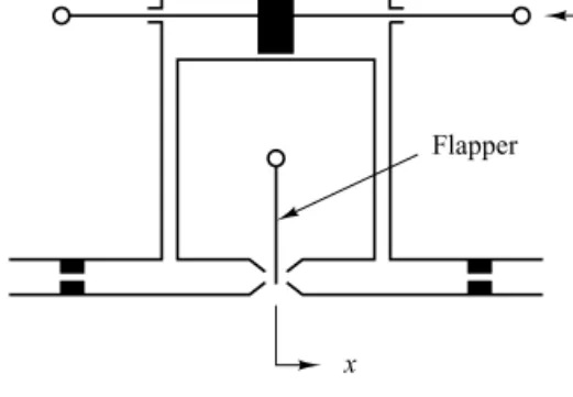
Summing Point. Referring to Figure 2–2, a circle with a cross is the symbol that indicates a summing operation. The plus or minus sign at each arrowhead indicates whether that signal is to be added or subtracted. It is important that the quantities being added or subtracted have the same dimensions and the same units.

Branch Point. Abranch pointis a point from which the signal from a block goes concurrently to other blocks or summing points.

Block Diagram of a Closed-Loop System. Figure 2–3 shows an example of a block diagram of a closed-loop system. The output C(s)is fed back to the summing point, where it is compared with the reference input R(s). The closed-loop nature of the system is clearly indicated by the figure. The output of the block,C(s)in this case, is obtained by multiplying the transfer function G(s)by the input to the block,E(s).Any linear control system may be represented by a block diagram consisting of blocks, summing points, and branch points.

When the output is fed back to the summing point for comparison with the input, it is necessary to convert the form of the output signal to that of the input signal. For example, in a temperature control system, the output signal is usually the controlled temperature. The output signal, which has the dimension of temperature, must be converted to a force or position or voltage before it can be compared with the input signal.

This conversion is accomplished by the feedback element whose transfer function is H(s), as shown in Figure 2–4. The role of the feedback element is to modify the output before it is compared with the input. (In most cases the feedback element is a sensor that measures

+–

a a – b

b Figure 2–2 Summing point.

(30)

the output of the plant. The output of the sensor is compared with the system input, and the actuating error signal is generated.) In the present example, the feedback signal that is fed back to the summing point for comparison with the input is B(s) =H(s)C(s).

Open-Loop Transfer Function and Feedforward Transfer Function. Refer- ring to Figure 2–4, the ratio of the feedback signal B(s)to the actuating error signal E(s)is called the open-loop transfer function. That is,

The ratio of the output C(s)to the actuating error signal E(s)is called the feed- forward transfer function, so that

If the feedback transfer function H(s)is unity, then the open-loop transfer function and the feedforward transfer function are the same.

Closed-Loop Transfer Function. For the system shown in Figure 2–4, the output C(s)and input R(s)are related as follows: since

eliminatingE(s)from these equations gives

or

(2–3) The transfer function relating C(s)toR(s)is called the closed-loop transfer function. It relates the closed-loop system dynamics to the dynamics of the feedforward elements and feedback elements.

From Equation (2–3),C(s)is given by C(s) =

G(s)

1 + G(s)H(s)R(s) C(s)

R(s) =

G(s) 1 + G(s)H(s) C(s) = G(s)CR(s) - H(s)C(s)D

= R(s) - H(s)C(s) E(s) = R(s) - B(s) C(s) = G(s)E(s) Feedforward transfer function =

C(s)

E(s) = G(s) Open-loop transfer function =

B(s)

E(s) = G(s)H(s)

Section 2–3 / Automatic Control Systems 19

R(s)

B(s) E(s)

G(s)

H(s)

C(s) +–

Figure 2–4

Closed-loop system.

(31)

G₁(s)

G2(s)

G₂(s)

C(s) R(s)

C(s)

C(s) R(s)

R(s)

+ +

G1(s)

G2(s) +–

(a)

(b)

(c) Figure 2–5

(a) Cascaded system;

(b) parallel system;

(c) feedback (closed- loop) system.

Thus the output of the closed-loop system clearly depends on both the closed-loop transfer function and the nature of the input.

Obtaining Cascaded, Parallel, and Feedback (Closed-Loop) Transfer Functions with MATLAB. In control-systems analysis, we frequently need to calculate the cascaded transfer functions, parallel-connected transfer functions, and feedback-connected (closed-loop) transfer functions. MATLAB has convenient commands to obtain the cascaded, parallel, and feedback (closed-loop) transfer functions.

Suppose that there are two components G₁(s)andG₂(s)connected differently as shown in Figure 2–5 (a), (b), and (c), where

To obtain the transfer functions of the cascaded system, parallel system, or feedback (closed-loop) system, the following commands may be used:

[num, den] = series(num1,den1,num2,den2) [num, den] = parallel(num1,den1,num2,den2) [num, den] = feedback(num1,den1,num2,den2) As an example, consider the case where

MATLAB Program 2–1 gives C(s)/R(s)=num兾den for each arrangement of G₁(s) andG₂(s).Note that the command

printsys(num,den)

displays the num兾denCthat is, the transfer function C(s)/R(s)Dof the system considered.

G₁(s) = 10

s² + 2s + 10 = num1

den1,

^G²^(s) ⁼ _s ₊⁵ ₅ ⁼ ^num2_den2

G₁(s) = num1

den1,

^G²^(s) ⁼ ^num2_den2

(32)

Section 2–3 / Automatic Control Systems 21 Automatic Controllers. An automatic controller compares the actual value of the plant output with the reference input (desired value), determines the deviation, and produces a control signal that will reduce the deviation to zero or to a small value.

The manner in which the automatic controller produces the control signal is called thecontrol action. Figure 2–6 is a block diagram of an industrial control system, which

MATLAB Program 2–1 num1 = [10];

den1 = [1 2 10];

num2 = [5];

den2 = [1 5];

[num, den] = series(num1,den1,num2,den2);

printsys(num,den) num/den =

[num, den] = parallel(num1,den1,num2,den2);

[num, den] = feedback(num1,den1,num2,den2);

10s + 50

s^3 + 7s^2 + 20s + 100 5s^2 + 20s + 100 s^3 + 7s^2 + 20s + 50

50

s^3 + 7s^2 + 20s + 50