Motivation and Background
Small Body Exploration for Science, Economics, and Humanity
For scientific, economic and humanitarian reasons, we seek to visit, land and sample small bodies. Small bodies are economically valuable for extracting rare materials and enabling long-duration missions in the outer solar system.
Meeting the Challenges: Proximity Maneuvers and Landing
With smaller size and without extensive material differentiation (i.e., separation of dense material into the core of the body), rare metals are readily available on small bodies. NASA and international partners (ie, the International Academy of Astronautics) have dedicated significant resources to planetary defense: the field that monitors and investigates possible collisions of small bodies with Earth.
Dangers of Uncertainty in the Dynamics
Where ∇2 = ∇ ∇ is the second partial derivative of the spatial variables (that is, the Laplace operator), ∇ is the divergence with respect to the spatial variables, and . Since the gravitational field is the most prominent part of the dynamics, we will focus on estimating this field.
Core Problem: Developing an Efficient Gravity Model for Spacecraft
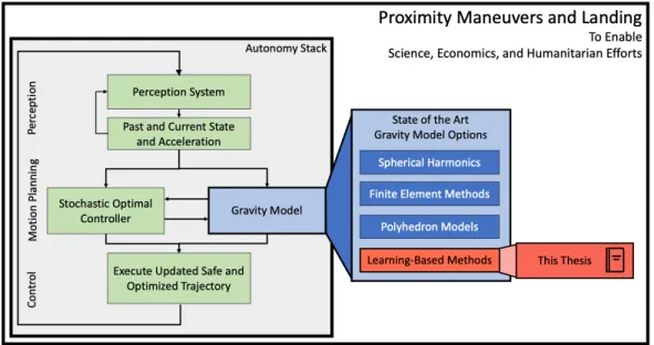
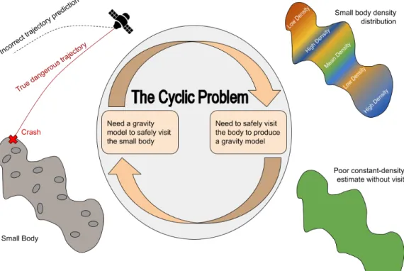
The efficiency of the gravity model reflects (1) a sufficiently accurate model and (2) a model that the optimizer can evaluate quickly enough. At the heart of the issue of developing a gravity model is its cyclical nature; it's a chicken-and-egg problem.
Contributions of the Thesis: New Methods in Trajectory-Only Learned
Furthermore, to produce a more detailed spherical harmonic model, we simply add an additional harmonic term (i.e., the complexity scales as 𝑂(𝑚)). The Hill sphere represents the sphere through which the gravitational influence of the secondary (eg an asteroid) begins to overtake the gravitational influence of the primary (eg the sun). The last constraint (Eq. 5.5) sets the boundaries of the trajectory (i.e. the trajectory starts at the spacecraft's current state and ends at the destination state).
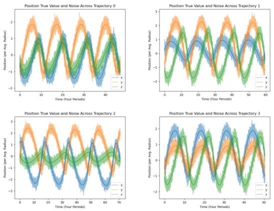
Comparison of Gaussian Process Model performance over data volume (i.e. the number of data points in the training data) and noise level (i.e. the noise added to the true trajectory training data. Since the noise is large (e.g. Figure 6.1), the inputs and outputs themselves do not maintain Lipschitz continuity. Consider if we examine a new position close to the trajectories or even the same input position but without the noise (shown as the red X). The point is not actually inside the training domain.
So we need to extrapolate to determine the acceleration at the new point (ie the red X is not in the light blue band). When the gravity model polyhedron is outside the shape polyhedron, we have a positive gravity anomaly (ie the material is denser than expected).
Objectives
Physics Engine for Trajectory-Only Learned Dynamics
Physics Engine Architecture
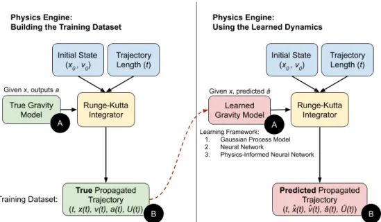
We use the true gravity model to build the training trajectory dataset (left side and green boxes). We then use the learned gravity model to build the predicted trajectory data set (right side and red boxes).
Gravity Model Trade-Offs
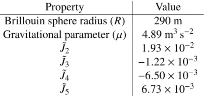
Finally, the spherical harmonic expansion is only valid outside the bounding sphere (also known as the Brillouin sphere, see Chapter 4 for more details). Therefore, for the purposes of this thesis, the expansion of zonal spherical harmonics is correct (Table 3.1).
Zonal Spherical Harmonics
Therefore, the expansion of zonal spherical harmonics is the right fit for the physics back end of the project: very versatile, computationally favorable, quite realistic, and quite available. The zonal harmonic terms are presented in equations where 𝐾 = 𝜇𝐽˜
The full derivation of the acceleration from the zonal spherical harmonic terms is presented in Appendix A.
Physics Engine Equations of Motion
We include the control constraint equation 5.4 to check that the controls are mechanically feasible (i.e., the controller does not require the spacecraft to exceed its mechanical propulsion or steering capabilities). We can provide a contrast between the first set of Gaussian Process Models (ie, Figures 6.4 and 6.5) and Neural Networks (Figures 7.1-7.3). If we probe a new position (ie, the red X), the new point is well within the training domain (ie, the red X is within the light green region).
When the gravity model polyhedron is inside the shape polyhedron, we have a negativity gravity anomaly (ie the material is less dense than expected, so we need a smaller volume of material to reach the measured field for the same density) .
Small Bodies through the Lens of Asteroid 101955 Bennu
Upper Bound on Validity: The Hill Sphere
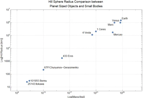
The hill sphere is an upper limit as other disturbances, such as solar radiation pressure will rise-. For reference, we have plotted the hill-sphere radii for various solar system bodies using data from Wolfram Alpha (Figure 4.1). Basically, in a third, this makes the power law in equation 4.1 where the mass𝑚 varies much more than the semimajor axis or eccentricity 𝑒.
Lower Bound on Validity: The Brillouin sphere
As fairly large terrestrial bodies, Venus, Earth and Mars are separated from the other objects. Mercury, the last terrestrial planet is separated from the rest by a similar Hill radius to 1 Ceres (a dwarf planet and the largest asteroid belt object). The other small bodies of Figure 1.1 are not included as their masses are not well known.
Zonal Harmonic Dominance within the Region of Validity
Even without physically informed learning (next section), the neural network with spectral normalization is able to approximate the dynamics about as well as the best test cases of the Gaussian process model. In the section on the Gaussian process model, we observed how the predicted propagated trajectories differ due to the model's inability to generalize the dominance of the point mass term beyond the training data. A comparison of the true potential with the predicted acceleration along with the associated error is shown in Figure 8.2.
In particular, the predicted accelerations of the physics-informed neural network (Figure 8.3) perform much worse than the most similar method: test case 3 of the neural network (Figure 7.3).
Methods for Trajectory-Only Learned Dynamics within Stochastic
Methodological Consistencies across Learning Frameworks
From a learning framework perspective, we start with a training dataset from past trajectories (for more details on data generation and the physics engine, please see Chapter 3). With the training data, the learning framework develops a model that approximates the underlying dynamics that generated the training data. Third, we evaluate the learning frameworks with two methods: (1) the accuracy of the trained dynamics model.
We do not need to explicitly test the generalizability of the learned dynamics outside the region near the trained trajectories as the error build-up in the propagated trajectories moves the gravity model evaluation outside the trained region, although this may be done in future work via a test trajectories pattern from a different initial state than the training trajectories.
Methodological Differences across Learning Frameworks
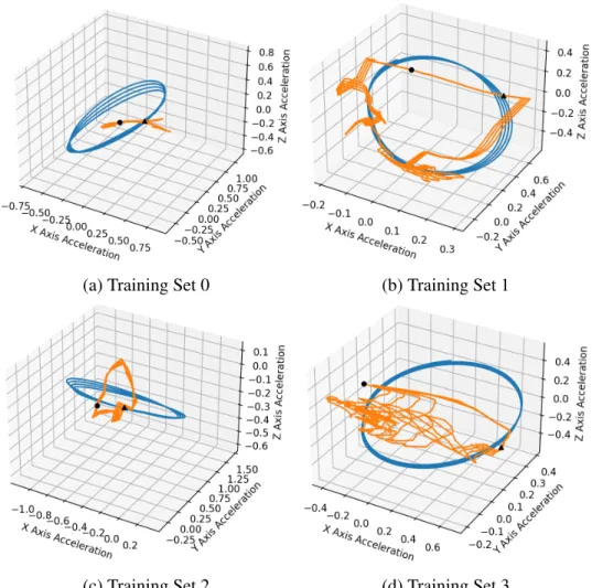
The accelerations predicted by the Neural Network (orange) do not accurately approximate the true accelerations (blue). Thus, the Neural Network predicts accelerations (shown in orange) that are either uniformly zero (training set 0 and 2) or fall along a line (training set 1 and 3). In contrast, the Gaussian Process Model appears to capture more of the variability, while not being as accurate overall (see subfigure (a) of Figure 6.4 and subfigure (a) of Figure 6.5).
In general, the Gaussian process model and neural networks outperform the physics-informed neural network.
Gaussian Process Model Frameworks
Base Orbits
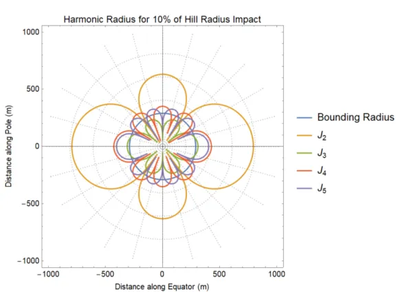
We select the arbitrary starting point for the integrator from a user-specified Keplian orbital element range (the starting point is based on the Keplian osculating orbit, but the orbit itself is not Keplerian due to the higher-order terms). For our primary set of base orbits, we select ˜𝑎 for the semi-major axis, 𝑒 for the eccentricity, and the fully defined range for the inclination, the longitude of the ascending node, the argument from periapsis, and the true anomaly. The ranges of the orbital elements are chosen so that the orbit is so close to the body that the higher-order terms in the expansion (e.g., 𝐽 .. 5) play an appreciable role (see Chapter 4 and specifically Figure 4-2).
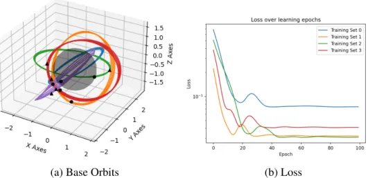
Four lanes are selected for training and an additional lane is selected for testing (Fig. 6.2).
Gaussian Process Model Training and Evaluation
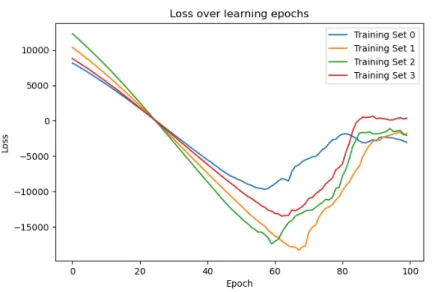
For all training orbits, the loss drops rapidly before increasing and leveling off at 100 epochs (Figure 6.3). To visualize the change in acceleration during the trajectory, acceleration vectors for actual accelerations and predicted accelerations are drawn in three-dimensional space (Figures 6.4 and 6.5). In this case, all orbits are spread by the same length of time, giving four thousand data points (each in R3).
This long horizon spread is outside the normal planning length and represents the extreme of the use-case for the learned dynamics.
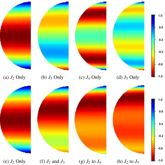
Comparison of Gaussian Process Model Across Different Harmonics 44
With the reduced noise, the neural network provides a fairly good approximation (orange) of the actual accelerations (blue). As with the Gaussian process model, the neural network does not encompass the full dynamics. With this in mind, the Gaussian process model significantly outperforms the neural network in cases where there is noise.
The loss appears to converge faster than the Gaussian Process Model and Neural Network cases.
Neural Network Frameworks
Neural Network Training and Evaluation
Furthermore, the predicted accelerations are not continuous (i.e., a small change in Table 7.1: Neural network training cases to illustrate the underlying limitations and the impact of spectral normalization. Test cases Noisy data Spectral normalization 1 Yes (Noisy) No (No spectral normalization ) 2 Yes (Noisy) Yes (Spectral normalization included) 3 No (No noise) Yes (Spectral normalization included). Since the spectral normalization is not included, the output does not preserve Lipschitz continuity. input position𝑥® gives a large change in acceleration ).
The neural network produces a continuous function (as the spectral normalization enforces) that moderately matches the real data.
Comparison and Contrast between the Neural Network and Gaussian
Since a Physics Informed Neural Network is fundamentally a subset of the larger family of neural networks, Physics Informed Neural Networks can also benefit from lower noise, large data volumes, and spectral normalization. This is shown as the middle panel in Figure 9.1 where the green points indicate samplings from the offline constant density multilevel model. One estimator may estimate the total mass of the body (and thus the point mass term), another.
To avoid matrix ill-conditioning under the hood of the Gaussian Process model, the function output (𝑎) must be in the same order as the input (𝑟) and close to unity.
Physics-Informed Neural Network Frameworks
Physics-Informed Neural Network Training and Evaluation
For a trajectory with sufficient coverage, the learning framework provides an unbiased estimate of the gravity field as it uses the measured acceleration data from the perception system (remember that the constant density polyhedron is a biased estimator as indicated in Section 3.2) and the perception data becomes higher given priority. The main problem with this method is that it does not overcome the computational complexity issues of the multilevel model. Investigating the best representation of the gravity model of a small body is an active research area and is beyond the scope of this thesis (Section 3.2).
We consider the arrangement where 𝑎 ∝ 𝑓(𝐺, 𝑀, 𝑟) where 𝐺 is the gravitational constant, 𝑀 is the mass of the primary, and 𝑟 is the position.
Concluding Remarks
Acceleration from Gravitational Potential
Note that just as force is the negative gradient of the potential energy, acceleration is the negative gradient of the specific potential energy according to Newton's second law. To obtain the acceleration, the derivative of specific potential energy is taken with respect to (𝑟, 𝜃, 𝜙).
Cartesian Conversion
Overview
Dimensionless Expressions in the Lowest Order System
Dimensionless Differential Equation
Even if they are not well constrained before flight, establishing these values and using them for normalization provides an essential method of comparing gravity models across bodies, avoids numerical ill-conditioning, and more naturally captures the magnitude of the problem. Since the parameter𝐾 is shared over each of 𝑎𝑥,𝑎𝑦 and𝑎𝑧, we label (for convenience in calculation), ˜𝐾 defined via equation C.15. Note that ˜𝑟 is usually between 1 (at the mean radius) and 100 (around the Hill sphere limit, depending on the mass of the object).
Therefore, we prevent bad conditioning, since the position, velocity and acceleration data are of the same order of magnitude and almost the same.
Summary and Key Takeaways