Magnetism in an Amorphous Fe-Pd-P Alloy System

Thomas E. Sharon

In Partial Fulfillment of the Requirements for the Degree of

Doctor of Philosophy

· California Institute of Technology Pasadena, California

1971

(Submitted May 10, 1971)

To Jerri, Tommy, and Michael

Professor Pol Duwez and Dr. C. C. Tsuei. The technical assistance of C. Geremia, S. Kotake, and J. A. Wysocki is also gratefully

acknowledged.

The author also wishes to thank the National Aeronautics and Space Administration, the International Business Machines Corpora- tion, and the Atomic Energy Commission for financial assistance which made this work possible.

Mossbauer effect in Fe 57 has been used to study the magnetic prop- erties of these materials. The hyperfine field distributions have

been determined from these experiments, as a function of composition and temperature. The results indicate that the eleetronic state of Fe in these alloys remains essentially constant throughout the composition range, and that the Pd d band is filled by electron transfer from phosphorus.

The variation of the magnetic transition temperature with composition has been determined by combining the Mossbauer effect results with complementary magnetic measurements. There is a sharp change in slope in this curve at x ~ 26. Below this concen- tration, the long range magnetic order which prevails in the higher Fe concentration alloys has broken down, giving rise to a more local ordering.

The Mossbauer effect results confirm the existence of weakly coupled Fe atoms in all the amorphous Fe-Pd-P alloys. These atoms reside in low effective fields, and can participate in the

spin-flip scattering process which produces a Kondo effect (resistivity.

III

A.

B.

c.

Preparation of Alloys

Mossbauer Effect Apparatus

Magnetic Transition Temperature Determination Study of Magnetic Properties Using the Mossbauer Effect -in Fe 57

A.

Hyperfine Interactions 1.

2.

3.

General Discussion

Electrostatic Hyperfine Interactions a. Isomer Shift

b. Quadrupole Splitting

·Magnetic Hyperfine Interactions a ^o Pure Magnetic Coupling

5 6 11

12 12 12 14 16 18 23 23 b. Combined Electric and Magnetic Coupling 23 B. Interpretation of Effective Magnetic Field at

the Nucleus L

2 ..

Contributions to the Hyperfine Field Relaxation Effects

25 25 27

2. Low Temperature Results

3. Analysis of Mossbauer Data Near the Transition Temperature

B. Variation of Transition Temperature with Fe Concentration

V. Discuss.ion

A.

Mossbauer Effect

1. Electronic Configuration of Fe in the Fe-Pd-P Amorphous Alloys

2 •. Asymmetry of Mossbauer Spectra

3 ^Q Variation of Hyperfine Field Distribution with Fe Concentration

a. Discussion of possible Pd d band polarization

b. Nature of the hyperfine field distribution:

relation to Kondo effect

4. Variation of Hyperfine Field Distribution with Temperature

35

60

63 .

79

79

83

84

84

90

97 .

VI

B.

Magnetic Properties

1. High Fe Concentration Alloys: x

>

^{2 5}

106 106 a. Discuss ion of magnetization results 106

2.

b. Comparison with theoretical treatments 109 Low Fe Concentration Alloys: x

<

^{2 5 115}

a. Evidence against superparamagnetism 115 b. Critical concentration effects 122 c. Nature of the magnetic state: Comparison

with the Au Fe system

d. Mechanism for magnetic ordering

126 131 3. Relation of Amorphous Fe-Pd-P Alloys to

Related Systems Summary and Conclusions

133. 139 References 143

over a decade ago, only in the last few years has the subject become an area of active experimental research. The existence of amorphous ferromagnets has been confirmed by conventional magnetic measure- ments (Z-S) and supporting Mossbauer effect data(6 ). Thus far the problem of magnetism in an amorphous alloy system {one in which the concentration of the magnetic element can be varied) has ·received less attention(7' 8 ). This is partly due to the. fact' that success in obtaining an amorphous structure has usually been limited to a rather narrow. composition range.

In order to make a meaningful study of the composition depen- dence of the magnetic properties of an amorphous alloy system, it is essential that a continuity of structure extends throughout the composition range. Although an amorphous material has no long range order (translational symmetry), it does possess definite structural properties based on its short range order. These are reflected in the radial distribution function (RDF) which is obtained from x-ray diffraction analysis, and form the basis for any discussion of the properties of an amorphous alloy. This requirement of

recently been studied by Maitrepierre(9.' ¹ O). It was shown that alloys of composition FexPd80 _xP20, where 13'< x< 44, can be quenched from the liquid state into an amorphous state using the "piston and anvil"

technique( 11). It was found from the radial distribution function data that the short range order in these alloys is continuous with respect to variation in the iron concentration, and that iron a~d palla- dium appear to substitute freely in this structure. Maitrepierre has suggested that the short range order in these alloys is based on the kind of structural units found in the metal rich transition metal

. (12)

phosphides {Pd3P or Fe3P) . In preliminary magnetization measurements, the saturation moment in a field of 8. 4 kOe and at 4. 2°K decreased in roughly a linear fashion from 2. 1 µB{Fe44Pd 36i=>20 ) to 0.6µB{Fe

13Pd

67P20). The higher iron concentration alloys were judged to be ferromagnetic by conventional criteria, but the low iron concentration alloys (x

<

2 5) showed a more complex behavior.

No Curie point could be defined from the magnetization data, and the effective moment in the paramagnetic region was quite large

(µeff ^{r J} 6 µB) • . These observations led Maitrepierre to suggest the existence of "superparamagnetisn1¹¹ in these alloys.

tions~ This is surprising because normally, in a crystalline system, only a few atomic percent of the magnetic impurity causes correlations between the spins which suppress the spin-flip scattering responsible for the Kondo effect. If the phenomenom of the resistivity minimum is really due to this process, this suggests that the correlations between neighboring spins in an amorphous material are significantly reduced compared to the crystalline state ^o

In the present work, a more detailed study of the magnetism

in this amorphous alloy system has been carried out, utilizing the Mossbauer effect and other magnetic measurements. There are several reasons for applying Mossbauer spectroscopy to the study of the magnetic properties of these amorphous alloys. This method permits one to examine the properties of single atoms, rather than complicated assemblages of atoms as in magnetization measurements.

The latter results are difficult to interpret if a complicated and perhaps unknown spin arrangement exists. Bulk magnetic measure- ments also cannot answer the question of whether all the moments are aligned to the same extent, or whether there is a continuous

quite valuable.

A second important reason for applying the Mossbauer technique is that no external field need be applied to the sample. The bulk

magnetic properties of a material are greatly influenced by such factors as domain structure, grain size, heat treatment, and many

other such effects. At present these factors are poorly understood for amorphous materials. In the Fe-Pd-P alloys, for example, even in the highest field (8. 4 kOe) and lowest temperatures (4. 2°K) used, the alloys appeared magnetically unsaturated(9). This means that the conventional techniques( 14) used to find the zero field magnetization, which is the quantity of real interest, are either inapplicable or of questionable accuracy. Furthermore, the application of large

external fields is undesirable because the microscopic spin ordering may change in response to this perturbing influence.

In the following, it will be shown how a Mossbauer effect study,

combined with complementary data fror.n other magnetic measure- ments, can greatly clarify the nature of the magnetism in this amorphous alloy syste.m.

from the liquid state using the "piston and anvil" technique(II).

Initially, appropriate quantities of iron (99. 9% purity), palladium (99. 99 % purity), and reagent grade red amorphous phosphorus powder were combined into briquets by a sintering process. These were then induction melted in an argon atmosphere and drawn into 2mm rods. The rods were then broken into pieces of appropriate size

for use in the quenching process. Full details of the alloy preparation may be found elsewhere(9, 1 O).

Because actual cooling rates rnay vary from sample to sample, each sample was carefully checked by a step-scanning diffractometer to ensure that only the broad bands indicative of an amorphous

structure were present. If a sample showed any weak Bragg reflect- ions superimposed on this background, it contained some crystalline phase and was rejected for use in further experimental work.

The resulting quenched samples are foils approximately 2 cm in diameter and 40- 50µ thick. For use as Mossbauer absorbers, the foils are somewhat thick. This results in high absorption and a relatively small resonant effect. It was thought unwise to thin the foils by mechanical or chemical treatment, however, because of the

chemical analysis after sintering(9). It was found that the actual compositions of all three elements were within 0. 5 at.% of the nominal ones. The small weight loss after melting (< • 2%) also indicates that it is reasonably accurate to designate the samples by their nominal compositions, hence we do so in any further discussion.

B. Mossbauer Effect Apparatus

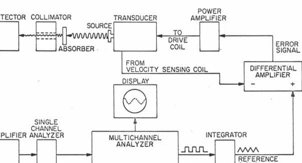
The Y-ray resonance absorption spectra were collected using the system illustrated schematically in Fig. 1. Gamma rays are emitted from a radioactive isotope (called the source), which in the present case is 10 mCi of Co 57 embedded in a Cu matrix. These photons are partially absorbed by any Fe 57 isotope within the sample·

(the absorber), and those which pass through are collimated and then detected with a gas filled proportional counter.

A current pulse proportional to the energy of the Y-ray is produced whenever a photon is detected. This pulse is amplified and then analyzed for energy by a single channel analyzer (SC~).

Only those photons whose energy corresponds to the 14. 4 ke V recoil- less transition are of interest for the resonance absorption spectrum.

DETECTOR COLLIMATOR

ABSORBER.

SINGLE CHANNEL AMPLIFIER ANALYZER

FROM

TO DRIVE

COIL

POWER AMPLIFIER

ERROR SIGNAL

VELOCITY SENSING COIL DIFFERENTIAL AMPLIFIER DISPLAY

0 v

MULTICHANNEL ANALYZER

INTEGRATOR

REFERENCE SIGNAL

+

Fig. l. Schematic· diagram of Mossbauer effect apparatus.

by an operational amplifier_, and then used as the reference signal to drive the velocity transducer which produces the Doppler shift

of the y-ray. This transducer is of the type described by Kankeleit( 15).

While the velocity transducer is producing a parabolic motion of the source (corresponding to a triangular velocity wave), a clock inside the multichannel analyzer opens one channel after the other for 100 µ, sec intervals. At the end of 512 x 100 µ sec, the process repeats itself. The actual motion of the source is sensed by a

pickup coil . which relays the information to a differential amplifier.

The reference signal is compared with the actual velocity signal, and an error signal is produced which forces the transducer to accurately follow the triangular velocity wave. The only significant deviation occurs at the turning points of the motion, where the relative error is about 1

%. ·

For use as absorbers in the Mossbauer experiments, the foils were cut into circular discs approximately

t"

in diameter. Experi- ments at room temperature, where a sin1ple two peak spectrum is observed for all but one of the compositions, required data collection

required that data be collected for a longer period. Hence for all but the liquid He experiments data were collected for several days.

The statistics for the liquid He experiments are noticeably poorer due to the reduced data collection time.

In order to study the samples at several different temperatures,

liquid helium and nitrogen, as well as dry ice-acetone slushes and ice - water solutions, were used. These coolants provided tempera- tures of 4.2°K, 77°K, 194°K, and 273°K re~pectively. Room

temperature experiments correspond to 29 5°K. Hence a wide range of temperatures is available to study the effects of temperature on the Mossbauer spectrum. ·Above room temperature a specially designed oven was used to provide continuous temperature control with a stability of about ±" 0. 5°K.

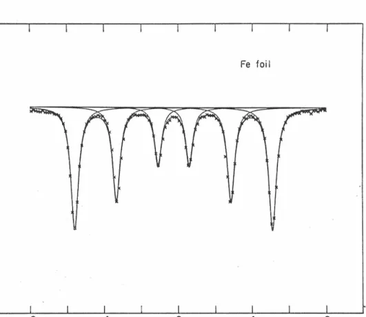
After each set of experin1ents an Fe foil was used to provide the velocity calibration (Fig. 2). The data were least squares fitted to a six peak spectrum and the line splittings of Preston et al(l6) were used to calculate the full scale velocity. According to their measurements, the separation of the outer peaks corresponds to

10. 657 mm/ sec.

0 z i= (L

0::

0 (/)

~ w >

~

_J

w a:::

.-8

Fe foil

-4 0 4 8

. VELOCITY ^(mm/sec)

Fig. 2. Example of velocity calibration spectrum taken with a • 001¹¹ Fe foil.

Since it is desirable to be able to locate the transition temperatures of samples which may fall in the intermediate temperature ranges, complementary methods were used to detect magnetic transitions.

The two techniques used rely on the drastic change in the bulk magnetic properties of a sample as it undergoes a magnetic ordering ^o In one method the sample was cut into the shape of a donut and many turns of fine wire wrapped around it to increase its inductance. This toroid was then used as an inductor in an LC 'oscillator. If the

frequency of oscillation is measured as a function of temperature, the magnetic transition can be easily recorded by taking readings from a frequency meter ^o Only the toroid is in the low temperature dewar, so that the change in frequency reflects only the change m its inductance. In the second method use was made of a V<?_ry sensitive bridge designed for detecting superconducting transition temperatures(l?). This system is capable of detecting transitions in only a few milligrams of superconducting material. Because the coils in the bridge circuit are balanced at low temperatures, its upward tempe.rature range extends only to about 30°K.

1. General Discussion

The great value of the Mossbauer effect in solid state physics arises from the ability to resolve the very small (-10- 8 eV) energy differences of nuclear energy levels. These perturbations, known as hyperfine {hf) splittings, are caused by the inter action of the nuclear magnetic and quadrupole moments with the surrounding elec- tronic charge and spin distributions. They are observable only if the linewidth of the recoilless gamma ray is 'small compared to these characteristic energies.

In Fe57 ,· for example, the decay scheme of the parent isotope C 57 . h . F. .

3{ 18)

o is s own in ig. . · . The isotope Co57

has a half life of 270 days, which makes it a very convenient source. It decays through electron capture to one of the higher excited states of Fe57. The Mossbauer transition involves an excited state of spin 3/2 (negative parity) and a ground state of spin 1/2 (also negative parity) •. The transition is almost completely magnetic dipole in character. Since the excited state has a lifetime of approximately 1

o-

7 sec, the linewidth of the emitted gamma is

Fig. 3.

Co⁵⁷ Decoy Scheme

706.4

366.8

136.4 5

2

9% 91%

14.4 3

2

,-

0 2

keV Irr

Decay scheme of Co 57 ..

T₁₁₂=0.98x10-¹ sec

The Mossbauer transition is indicated by the .dashed arrow.

In Mossbauer effect studies the energy of emitted photon from the source is Doppler shifted an amount ~ E₀ {E

0

=

14. 4 ke V).

To obtain shifts in the range of the hf interactions, velocities in the range 1-10 mm/ sec are usually involved.. It is customary to express all energies in terms of the velocity required to produce ,the correspond- ing Doppler shift. For example, the linewidth of the emitted ,gamma ray is 0. 09 5 mm/ sec in these units. If another Fe 57 nucleus absorbs this photon, the resulting linewidth when plotted versus velocity will have a theoretical value of

2r

⁼ 0.19 mm/sec. In practice the observed linewidth is always significantly greater than this due to several broadening mechanisms. ,

2. Electrostatic Hyperfine Interactions

It is well known that the nucleus is not a point charge but has a finite radius of the'order of 10-13 cm. If we consider the energy of this nuclear charge distribution p(x) in the electrostatic potential V(x) produced by the surrounding charges, the expression for its energy is(l9)

( 1)

parent aton1, as well as any surrounding charges external to the atom. Since this energy is expected to be small compared to the nuclear transition energy, we may expand V{x) in a power series about x

=

0 and insert into Eq. ( 1)

3 3 ~

Eel

=JP

(X) [ V(O)

+I:

Vixi

+ ~ I: I:

^{V .. x.x.}

^{+ ...} Ja

^{3x (2)}

. i

=

^{1 'i}

=

^{1 j}

=

^{1 lJ 1 J .}

where

v ..

lJ

Vi=

(:~J

^X=O

v .. = ( a2v )

lJ

ax.ax.

1 J x=O

is known as the electric field gradient {efg). · To simplify this expression note that

j

p(X) d 3x = Ze and that

v ..

lJ is a symmetric matrix. Hence principal axes for the last term may be chosen such that

3 3

;: Z eV(O)

+ L: ^{v. fp}

(X.)x. d 3x

+ i L: ^{v ..} fp(x}x~

^{d 3x}

^{+ ...}

· i

J'

^l

nJ

^{I- l}

i= 1 i= 1

(3)

may be neglected because the electric dipole moment of the nucleus is zero (parity is a good quantum number). It can be shown that all terms above the third are also zero(ZO). This leaves only

(4)

Rearranging slightly we get

3 3

Eel=

~I:

^vii

JP

^(X)r2d3x

^+~I:

ViijP (x) (xi2

-

i

^{r2)d3x (5)}

i=l i= 1

These terms are of great importance to what follows, and lead to the effects known in Mossbauer spectroscopy as the isomer shift and quadrupole splitting, respectively.

a. Isomer shift

The first term of Eq. (5) can be put in a more useful form by applying Laplace's· equation,

3

L:

Vii = - 4 ^7r p e 1 ( O)=

+

4 ^7r e

I

^{'11 ( 0 )}

^j

²

i= 1

(6)

I

^{'I'( 0) ( 2} is the total electronic density at the nucleus. Thus we have,

3 ⁽⁷⁾

2 7re

The net displacement ^t of the energy levels is therefore

where the subscripts e, g refer to the excited and ground states.

In Mossbauer experiments we observe the net shift of the absorption line between absorber and source, which is the isomer shift

b

To put Eq. (10) in conventional form we assume a constant nuclear charge density out to the nuclear radius R. Then

2 7r

ze

²

5 . ( 11)

For Fe57 , Re and Rg are very nearly equal, and Re< Rg•

Thus it is customary to write

Thus the final expression from isomer shift is,

increase in the charge density at the nucleus in the absorber will result in a decrease in the isomer shift, since AR/R is negativeo The isomer shift is sensitive to the electronic state of the Fe atom.

Although

I\{!

^{(O} f 2} is due to only s electrons which have nonzero wave function at the nucleus, a change in the number of 3d electrons will also have a large effect on the isomer shift, since the screening of the outer s electrons is affected by this change. Thus the isomer shift is a valuable indication of the chemical or valence state of the Fe atom.

b. Quadrupole splitting

A similar procedure for the second term of Eq. ( 5} can be carried out. Starting ·from

EQ

= t ~

L.,, ^{V ..} 11

JP

^{(x} (x.}l ^{2 - _!_ r}3 ^{2} d3x} i= I ·. ·

( 13}

we note that only s electrons have finite densities at the nucleus (in the nonrelativistic limit), and these produce a· spherically sym- metric potential. Therefore V xx

=

^{V yy}

=

^{V zz} for these charges·

and

bute to the electric field gradient causing the quadrupole interaction,

v

_xx

+v +v

_{yy zz}

= o

^(15}

For cubic symmetry, we have the immediate result that there is

no quadrupole splitting, since V _xx

=

^V _yy

=

^V _zz

=

^{0 from Eq. (15).}

For the case of axial symmetry (V xx

=

^V _yy ^{) , Eq. ( 13) 'reduces}

to

( 16)

The quantum mechanical expression for Eq. ( 16) follows from the fact that (2 0)

3m 2 - I(I+l) eQ

31 2

- I(I

+

1)

_ If ,

^{):c [}

^~

^{2 2}

^{J -}

where

Q-e

'l'II LJ ri (3cos 8i- l) '1'Ildr 1 dr 2 ..• drA . i= 1

(17)

is the expression for the quadrupole moment of the nucleus of A nucleons and spin I, and m is the quantum number for 1

2

• ·'II II is the wave function corresponding to the maximum projection

=

^{1 e2 q} Q 3m2

- I(I+ 1)

4 (18)

312 - I(I+ 1)

where eq

=

V zz is the conventional definition for the electric field gradient.

For the case of Fe57 where le= 3/2, Eq. (18) gives two energy levels

Fig. 4a illustrates this case for q

>

O~ The resulting Mossbauer spectrum consists of two peaks (of equal intensity for a powdered absorber) with separation !-?ae2 q Q J .

For the general case of nonaxial symmetry, the quadrupole Hamiltonian becomes

:H

= e2

q

a [

2 7] 2 2

J

Q 41 (21-1) . 3Iz - I(I + 1) +

Z

(I+ + I_ ) ⁽¹⁹⁾

v

-V

where ⁷⁷ = xx yy

v

_zz

I+ ^{= I}

±

i I

x y

te2qQ m +.l

-€~r

^{+~ 2}

±~ ²

:3 _J.. ² +l. +.l

e²qO 2

Ie• 2 _~Ee

1

2 2 I

-2 ^I

±2 -2

_ _l

-~

2

I I

-2 -2

~Ec;i ~Ec;i

+_!_ ₂ +.l

2

(a.) (b) (c)

Fig. 4 • . Nuclear energy levels of Fe 57

and resulting Mossbauer spectra: (a) Electric quadrupole

interaction. (b) Magnetic hyperfine interaction.

( c) Combined magnetic and electric quadrupole interactions with efg principal axis parallel to H.

however, the splitting is I

~

e2q QI [ 1

+

^{Tl 2}

I

3

Jt

and the eigen-

/\

states of HQ are no longer eigenstates of Iz (21) a The intensity of the two lines remains equal for a powdered sample, however, so the appearance of the Mossbauer spectrum is just as in Fig. 4a.

A measurement of the quadrupole splitting provides information about the electronic state of the Fe atom, as well as the effects of the local environment. Since there are two major sources of the electric field gradient - the charges on neighboring ions and the electrons in incompletely filled shells {3d for Fe), the two contri- butions must somehow be separated if a useful interpretation is to be made. This is sometimes possible by studying the temperature dependence of the quadrupole splitting. If the efg arises mainly

from internal electrons in unfilled shells, the temperature dependence is often quite pronounced because of the change in population of

the crystal field states. In a metal, however, the quadrupole splitting is usually insensitive to temperature and arises mainly

from the deviation of the local environment from cubic symmetry(ZZ)Q

magnetic moment is nonzero, then there is an additional term in the Hamiltonian representing this interaction

H A

M

- - µ, • H

-

Since

Ji =

^{g µ,N}

^{f (}

µN is nuclear magneton)

This simple Hamiltonian has the eigenvalues

where m is the quantum number corresponding to I . A good . z (20)

(21)

(22)

example of pure magnetic coupling is the spectrum of an ordinary Fe foil. Because of the cubic symmetry, the quadrupole interaction is zero and the energy levels are given by Eq. (22). Since

g

I

g

= -

^{l · 715} for Fe 57, the six line spectrum illustrated in g e

Fig. 4b results. (See also Fig. 2).

b. Combined electric and magnetic coupling

In noncubic magnetic materials there exist in general both electric qu~drupole and magnetic interactions. The resulting

In the most general case it is best to express each in terms of its

own favored axes, and then by using appropriate rotation operators to express both in a comn10n set of axes. This greatly complicates the analysis, since the eigenvalues and eigenvectors are no longer expressible in closed form. Only for special cases are closed form

solutions available. One such case, which will be of great import- ance to follow, is the problem of the axially symmetric efg with principal axis at an angle 0 with respect to the magnetic field direction< 23 ) ^e Then

E(m) = _ g µN Hm

+ (-

l)lml

+~

^e2

.{Q [

³

co~

²

e-

¹

J

⁽²³⁾

provided µH»

I

^e2.{Q

For 0

=

0, Eq. (23) reduces to the simple expression for collinear axes of the magnetic field and axially symmetric efg. In this case all four sublevels of the excited state are shifted by a magnitude

I

^{e2qQ J} with the resulting spectrum illustrated in Fig. 4c. The

4 .

more general case described by Eq. {23) has exactly the same appear- . d d th 1 t f b ^{I --} q ( 3 ^{C 0 S}

2e-

1 ) ^{l. S}

ance, pro ^{v i} e e rep acemen o q y q

- 2

The magnetic field at the nucleus is due to several factors.

. (24)

According to Marshall , it can be expressed as

where

H= H· t m

+

· H dipolar

+

H orbital

+

H c

H. _in t

=

^H _{applied -} ^DM _s

⁺

⁴ ₃ ^{tr M} _s

⁺

^H'

(24)

DM₈ is the demagnetizing field, and H¹ is the correction term to the 471'"

Lorentz field . -

3- Ms for non-cubic symmetry. When the external field is zero, the contributions from Hint are usually small and can generally be neglected.

The second term in Eq. (24) arises from the dipole interaction between the electronic and nuclear spins and is usually of the order of 1- 10 kOe. (2 3

)

The orbital term arises from the circulating current due to a nonzero angular momentum. If t.he angular mon1entum is quenched

-fl

( L

=

O), this term is zero. In metallic iron, however, this term has been estimated to be · +7 0 kOe (2 5).

core s electrons and 4s conduction electrons by the 3d magnetic electrons.. The contribution from the core electrons is directed in the oppooite direction to the magnetic moment of the atom, while the contribution of the 4s conduction electron polarization at the nucleus and the orbital contributions are positive. For metallic Fe the polarization of the core electrons is estimated to give a contribution of -(400-500)k0e. The expression for He is(26)

(2 5)

Marsha.ll{2 7) and others have shown that all the factors contributing to the magnetic field at the nucleus should be propor- tional to the magnetic moment of the parent atom. Hence a plot of the hyperfine field and magnetization should have identical variation in temperature. Experimentally it has been shown that for pure Fe{ZS) and for Fe Pd (Z9} alloys this is true to an excellent approx- imation. When the reduced hf field deviates considerably from the reduced magnetization, it usually occurs when Fe. is being used as a magnetic probe in a different magnetic host, for example NL Then the variations in exchange interaction between host-host pairs

considered to be parallel (or antiparallel) to the moment of the atom • . This moment is not a static quantity, however, because of various

relaxation processes (mainly spin-lattice and spin-spin) the electronic moment is in a constant "flipping" process as it changes its state.

If the frequency of flipping is much larger than the Larmer frequency

of the nuclear spin in its internal field, the nucleus will see only the average of this hyperfine field. For paramagnetic materials'. this should be zero. If on the other hand, the spin flip frequency is

comparable to or smaller than the nuclear Larmer frequency) a hyper- fine field may be observed even in a material with no magnetic order.

For this to be possible in practice requires very dilute magnetic impurities to minimize spin-spin interaction.

To minimize spin lattice relaxation, the ion should be in a S state to eliminate any coupling to the lattice through the spin- orbit interaction. Also the material should be non-metallic, to eliminate relaxation processes involving conduction electrons.

These conditions are met in very dilute Fe: Al 2

°"3,

where a hyper- fine splitting is observed at low temperatures in the paramagnetic state(30). In a metallic non-dilute magnetic host, however, relaxation

z

Another slightly different relaxation effect occurs in "super- paramagnetic" materials. These are substances in which there exist small clusters of magnetically coupled atoms. This could refer to a

0

very fine Fe or Fe

2

o

₃ powder ("" 100 A diameter particles), or perhaps to a magnetic phase precipitated out of a nonmagnetic matrix.

In any case one requirement for "superparamagnetisr.n" is that the particles are small enough to ensure that each is· a single domain. In these materials the magnetization vector in each particle undergoes a kind of Brownian motion due to thermal energy in which it is continuously changing its direction among the various possible easy directions of magnetization. This ensures that no hysteresis effects such as remanence or coercive force exist in superpara- magnetic materials (31).

It can be shown that the frequency corresponding to this process can be described by a relaxation time

T :

ro

^exp KV

kT (26)

where r

0 ~ ·10-9 sec, K is the anisotropy energy per unit volume,

particles maintain their magnetic alignment internally. These effects have been observed in many superparamagnetic systems(33- 36).

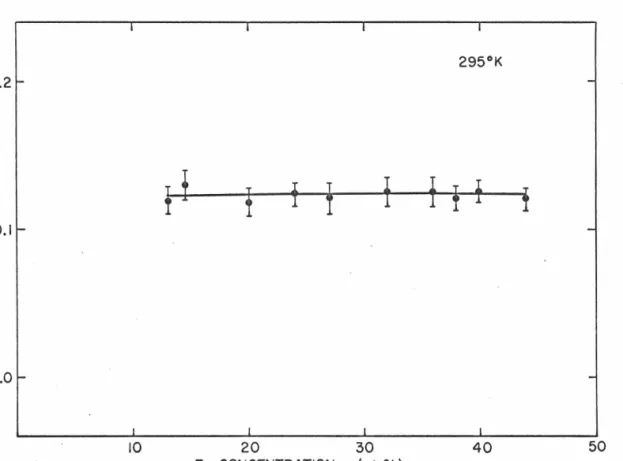
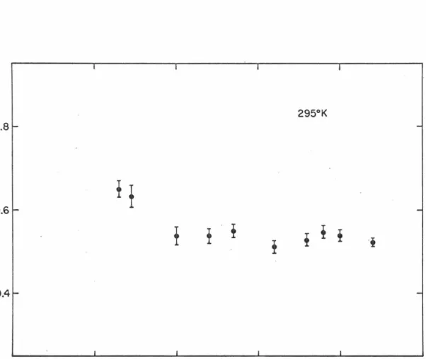
Typical Mussbauer spectra for the amorphous Fe-Pd-P alloys at room temperature (295°K) are shown in Fig. 5. As explained in Section III, a sufficient condition for the absence of quadrupole splitting is cubic symmetry at each Fe site. Since the amorphous alloys obviously do not satisfy this criterion, the two peak spectrum is expected . . At this temperature only the highest Fe concentration alloy (Fe 44Pd36P 20 ) shows evidence of magnetic splitting. The experimental data were fitted to two Lorentzian peaks of equal

areas. The widths were allowed to vary to allow for some correlation between isomer shift and quadrupole splitting, which would produce an asymmetrical spectrum. The width difference for almost all the samples was found to be quite small(< . 01 mm/sec), thus the

spectra are nearly symmetric.

Figures 6-8 show the parameters obtained by a least squares fitting using this approach. The large broadening observed (a line- width of 028mm/sec is obtained with the same source and a thin Fe foil) is characteristic of the large scatter in isomer shifts and field gradients which exist in the amorphous material. The values

z 0 f- CL 0:: 0

(/) m

<I:

w >

~ _J

w 0::

-2 -I 0 I

VELOCITY (mm/sec)

Fig. 5. Typical Mossbauer spectra for the amorphous

· FexPd80_xP 20 alloys at room temperature (295°K).

u <U

<

_E

.5

t-u....

I

(/)

a:: w

~ 0 (/)

w

~

295°K 0.2

f 1 ! ^f ! ^{! ! f ±}

0.1

0.0

10 20 30 40

Fe CONCENTRATION x (at.%)

Fig. 6. Isomer shift vs. iron concentration for the . amorphous FexPd80 _xP 20 alloys.

f

50

1.0

u <l>

<

_E

E l? z 0.8

I- I-

=:i 0...

Cf)

w _J

0 0...

:J 0.6 er 0

<!

:J 0

w

~

0.4

295°K

10 20 30 40

Fe CONCENTRATION ^{x (at.%)}

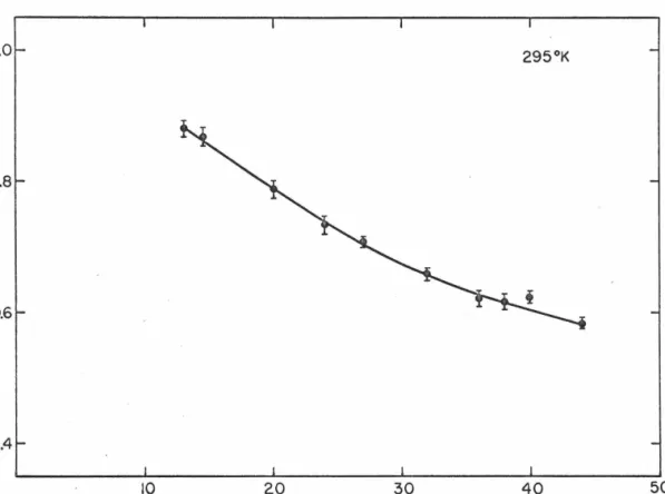
Fig. 7. Quadrupole splitting vs • iron concentration for the amorphous FexPd80_xP20 alloys.

50

u <l>

z

E E

0.8 -

- 0.6-

I

I I I I

295°K

l-o

~

! ! !

w z ::J

0.4 ^{I -}

I I I

10 20 30

Fe CONCENTRATION x (at.%)

Fig. 8. Linewidth vs. iron concentration for the amorphous FexPd80_xP 20 alloys.

I

40 50

data, since the linewidth depends on such factors as foil thickness and vibrational broadening which are not easily controlled.

2. Low Temperature Results

The problem of analyzing the Mossbauer spectrum of a magnetic material is greatly simplified by a knowledge of its structure. From this information one obtains the ·number of inequivalent Fe sites

{hence components in the s pe ct rum). In the crystalline case, one also obtains the point symmetries at each Fe site. This information is important because of the constraints imposed on the parameters used to fit the experimental data. Even with this knowledge, the problem of analyzing the ·absorption spectrum of a magnetic material with several sites per unit cell can be quite complicated, since a nonlinear least squares procedure with many parameters must be used. For a disordered alloy, the difficulty of the calculation in- creases immensely since the number of inequivalent sites actually becomes infinite. In the amorphous case, the difficulties may be expected to be even greater. Therefore, before discussing the analysis of the Fe-Pd-P Mossbauer spectra at low temperatures it may be helpful to briefly discuss two different approaches to the

Ni) in body centered cubic {bee) Fe. These alloys may be denoted by the form Fe X (the underscored element is the solvent or host

material), where X represents one of the other transition metals in the 3d series. In the bee structure, there are eight nearest neigh- bors (nn) and six next nearest neighbors (nnn}. Since the two

components form a random solid solution for low X concentration, -one can calculate the probabilities for various nearest and next

nearest neighbor configurations.. It was then assumed that the magnitude of the hyperfine field at a given Fe site depends only on the number of these impurity neighbors ·in the following fashion:

H{n, m)

=

H' {l - an - (3m)

where H' is the hyperfine field of pure Fe(330 kOe), and n, m are the number of nn and nnn impurities. A corresponding expression is used for the isomer shift. One then calculates the Mossbauer spectrum corresponding to each set of (n, m) values, weights it with the appropriate probability, and sums over the 63 possible configura- tions.

It was found that the ratio of

f3

to a which yields the best

for one nn, 6% for one nnn). Again these values do not depend greatly on the nature of the impurity.

The analysis is greatly simplified by the fact that there is no need to consider. the quadrupole coupling. This fortuitous circumstance stems from the fact that the introduction of one nn impurity produces a field gradient with its principal axis along the [ 111] direction.

Thus even though the quadrupole interaction is not absent, the factor [3 cos 2

e-

l] in Eq. (23) is zero because

th~

spins are aligned along a [ 100] direction. Next nearest neighbor effects are significantly smaller because of the screening of electrostatic effects in a metallic host such as Fe. It is evident that this approach begins to break down when there is an appreciable probability of two or more nn impurities.

This limits the approach to dilute impurities (< 10% X).

The other disordered alloy problem which is easily treated is the case of dilute Fe impurities in a cubic host. Here the best example is Fe Pd (29, 38). These alloys 1 which have the face

centered cubic (fee) structure, become ferromagnetic at exceeding low Fe concentrations (""'. 1

%

Fe). The environment around each

of these methods are clearly inapplicable because of the concentration range involved and the lack of symmetry. Therefore, a combined magnetic and electric quadrupole interaction of the most general kind discussed in section III must exist. The only a priori structural information is the averaged radial distribution function, which gives no information about the angular distribution about any given Fe atom.

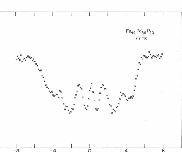
In light of these difficulties, the approach to be followed must rely heavily on the experimental results for clues in interpreting the observed spectra. A typical low temperature Mossbauer absorp- tion spectrwn for the Fe-Pd-P alloys is shown in Fig. 9. There are several observations of significance to be made. First, it is possible to distinguish six peaks, although they are greatly

broadened compared to the Fe foil spectrum of Fig. 2. A check of the line positions shows that they are in roughly the same ratio as observed for pure Fe. The inner peaks are noticeably sharper than the outer peaks~ Finally, aside from the small differences in

shape of the outermost peaks, the spectrum is nearly symmetric about its center. This last feature is quite surprising in view of the

z 0 l-o...

0::

0 (/)

~

w

>

~

_J

0:: w

-8

I

)(

)(

>l'- ^{)( ~}

~ ⁾⁽ )( >f<

)( )( )(

)(

)( )(

)( )(

)( )(

)( )(

I I I

-4 0

VELOCITY (mm/sec)

Fe44 Pd36 P20 77 °K--.

I 4

)(

)(

I

Fig. 9.· Low temperature Mossbauer spectrum for the Fe44Pd

36P

20 alloy.

I 8

broadens the peaks, rather than changing their positions. No further explanation was suggested for this effect, however.

If we also momentarily neglect the quadrupole interaction, the experimental data are consistent with a distribution of hyperfine fields in the alloy. The increased broadening from inner to outer peaks is consistent with this assumption, since each line would be broadened roughly in proportion to its displacement from the centroid of the pattern (see Fig. 4b}. From an approach based on Eq. (27), it is possible to see how a range of hyperfine fields could exist in an amorphous m'aterial. From the RDF, we know that in an amorphous material the nearest neighbor atoms are not at one precise separation,

but rather a shell of atoms exists whose width may be roughly 0.

s.R

(IO}. The second shell is less well defined. In Eq. (27), therefore, a and {J take on a range of values, depending on the

exact positions of the atom in the shells. In the amorphous Fe-Pd-P alloys, one of the dominant mecranisn~ affect~ng the hyperfine

field at an Fe atom is expected to be electron transfer from neighboring phosphorus atoms. By donating electrons to the 3d shell of the Fe atoms, their moment and hyperfine field will be reduced(6). We can

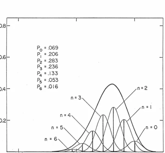
close packing (approximately 12 nearest neighbors) with 20% of the . sites randomly occupied by phosphorus. We then write

H {n)

=

H' { 1 - an) (28')

where only nearest neighbor effects are considered for .simplicityg in view of the fact that in amorphous materials short range effects are expected to be dominant. The value for H' is taken to be 300 kOe {appropriate to Fe Pd alloys); and

aH'=

18 kOe (a 6%

decrease for 1 nn P atom). The probabilities of the various hyper- fine fields are then given by the binomial distribution:

{29)

These values and their corresponding hyperfine fields are represented by the vertical bars in Fig. 10. To allow for the amorphous nature of the alloy,. we now allow ·a to take on a range of values. This

distribution may be assumed to be due to fluctuations in interatomic distances and next nearest neighbor effects. This is illustrated in Fig. 10 for .

J(

A a )²

I

a

=

0. 66, where {~a )2 is the mean square

0.8

0.6

-

^I

a..

0.4

0.2

100

P₀ = .069 P₁ = .206 P₂ = .283 P₃

=

.236 P₄ =.133 P₅

=

.053 p6

=

.016

n = 5

n

=

6

n=3

200 300

H (kOe)

Fig. lOo Illustration of possible hyperfine field distribution in an amorphous. material.

A such that the width of the peaks is given by

ri

= r

₀

c

ⁱ

⁺ x I

^Ei

I J

⁽³⁰⁾

where

I

Ei

I

is the displacement of the ith peak from the c~ntroid of the absorption pattern (isomer shift). This is the approach followed by Tsuei et a1(6) in discussing the amorphous Fe-P-C alloy. They used five sets of six peak patterns, and achieved a good fit of the experimental data.

For the amorphous Fe-Pd-P alloys, this approach was consid- ered but not used for several reasons. First, the number of variable parameters is quite large and these parameters often vary unpre- dictably. In particular, the intensities for the different six peak components do not always agree well with a binomial distribution.

The large number of parameters (31 for five sites} makes the nu- merical analysis quite lengthy and very expensive in computer time.

Secondly, the lack of detailed structure in the spectra of the Fe-Pd-P alloys makes it unlikely that a unique fitting based on a certain

number of sites can be achieved. In fact, the most that can probably

It was decided, therefore, to base the analysis of the Mossbauer spectra on a distribution of hyperfine fields. As a first attempt,

a Gaussian distribution of fields was assumed. This is equivalent in the simple model illustrated in Fig. 10 to replacing the top curve representing the sum of the components by a Gaussian curve of appropriate average value and width. This would appear to be a quite good approximation. Thus it was assumed that

P(H) = 1 exp [- (H-H)2

J

2~2 {31)

was the probability density function for hyperfine fields. A computer program was wriHen to calculate the corresponding Mossbauer

absorption spectrum, and a nonlinear least squares analysis was used to adjust H and ~ to best fit the experimental data. Using this approach it was found that the outer peaks could be fitted quite well, but the absorption in the central part of the spectrum was much greater than predicted by this simple model. This implies that

there are significant contributions to the absorption coming from Fe sites with small hyperfine fields. In other words, the distri-

the calculation, it is convenient to have an analytical form for P(H). It was found that the form of P(H) can be well represented by the following empirical formula:

1

P(H) a (32)

exp -

The two forms are matched in value at H

=

_. H ₀ and P(H) is then normalized numerically so that 1.;(H) dH

=

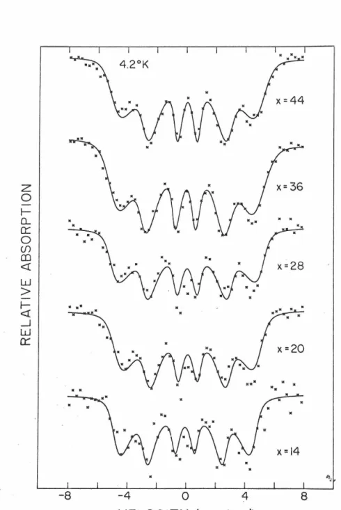
^1.

Typical. fittings achieved with this model are shown in Figs.

11-16, along with the hyperfine field distributions, and are quite good considering. that only 3 parameters are involved in the analysis.

This means that the actual P(H) distribution is quite well approxi- mated by Eq. {32). In Tables I-III the actual values for the

parameters and their estimated standard deviations are shown. In Tuble IV we present the average value

fr = f

00P(H) H d H and the

0

standard deviation /:J. H for the distributions at 4.

z°K.

^~His

defined by

z 0 I-

()_

0::

0 if)

co <!

>

w

I- ^{IC • •}

<!

_J

w

0:::

-8 -4 0 4 8

. VELOCITY (mm/sec}

Fig. 11. Mossbauer spectra of the amorphous FexPd

80_xP 20

· alloys at 4. 2°K. The experimental points are shown and the fitting based on Eq. (32) •

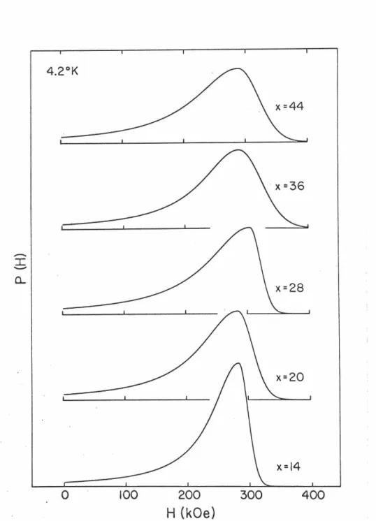
0 100 200 300 400 H (kOe)

Fig. 12. Hyperfine field distributions corresponding to the fittings of Fig. 11. The vertical scale is the same for all the curves.

z 0 I-Q_

0::

0 (f) Q)

<r:

w >

~ _J

w a::: _x=32

. x =24

-8 ^~4 0 4 8

VELOCITY (mm/sec)

Fig. 13.. Mossbauer spectra of the amorphous FexPd80_xP 20 alloys at 77 K. 0

I CL

0 100

x=32

200 300 400

H ( k Oe)

Fig. 14. Hyperfine field distributions corresponding fo the fittings of Fig. 13.

z 0 I- Q_

0:: 0

(f) Q)

<(

w >

~ _J

w 0:::

-8

194 °K x=44

..

_{M M}

x=32

-4 0 4 8

VELOCITY (mm/sec)

Fig. 15. Mossbauer spectra of the amorphous FexPd

80_xP 20 alloys at 194 K. 0

I

a..

0 100 200

H (kOe)

x =36

300 400

Fig. 16. Hyperfine field distributions corresponding to the fittings of Fig. 15~

TABLE I Parameters obtained from analysis of Mc5ssbauer Effect data at 4. 2°K based on Eq. {32). standard deviations are shown in parentheses. The symbols

b

and

r

refer to the average shift and linewidth, res pecti vel y. Composition b{rnm/sec)

r

{mm/sec) Fe44Pd36p20 0. 102 (. 017) 0 e 44 7 { • 04 7) Fe36Pd44P20 0.108 {. 016) 0.523 {.046) Fe28Pd52P20 0.085 {.030) 0. 5 5 3 {. 09 5) Fe24Pds6P20 0. 076 {" 020)

o.

444 {. 055) Fe20Pd60P20 0 e 08 0 { • 021) o.510 {.069) Fe 14Pd66p20 -0. 043 {. 052) 0 • 5 54 { • 1 8 1 ) H {kOe) 0 288. 4 (4. 5) 287.7 (3.8) 304. 9 { 13. 7) 296. 6 (4. 8) 284. 2 (6. 7) 283.2 {21.4) L\ 0{k0e) 17L8 {11.0) 146.6 {8.3) 167.0(17.1) 167. 6 {12. 5) 148.S{lLl) 106. 0 {26. 2)

TABLE II Parameters obtained from analysis of Mossbauer Effect data at 77°K based on Eq. (32). Comp~sition

b

(mm/ sec)

r

(mm/ sec) H 0(k0e) & 0(k0e) Fe44Pd36p20 . 0. 09 8 (. 009) 0.500(.027) 265.9 (2.4) 152. 0 (5. 24) Fe40Pd40P20 0.133 (. 005) 0.643 (.017) 257.4(1.7) 151. 8 (2. Fe36Pd44p20

o.

070 (. 011) 0.511 (.032} 248. 0 (3. 3) 183.7 (6.9) Fe32Pd43P20 0.111(.018) 0. 49 5 ( . 04 6) 194. 2 (6. 6) 210.4 (4.6)

TABLE III Parameters obtained from analysis of Mossbauer Effect data at 194°K, 273°K, and 295°K based Eq.· {32). Com posit ion b(mm/sec)

r

(mm/ sec) H 0(k0e)

£\

0{kOe} Fe 44Pd 36P 20( l 94°K) 0. 09 1 (.

b

1 5) 0.470(.039) 207.9(3.3) 154 o 1 ( 8. 8} Fe40Pd 40P 20( l 94°K) 0.092(.004) 0.464(.009) 191.5(1.0} 155.4(2.2} Fe36Pd44P20< l 94°K) 0.125(.037) 0.583(0145) 140.7(16.6} 211.6(38.7} Fe44Pd36P20{273°K) 0.138(.022} 0.560(.095} 133.4(9. 1) 165.0(19.4} Fe44Pd36P20(29 s°K) 0.129(.013) 0.511(.080} 87.,3(7.5} 142.l(?I.8)

TABLE IV Characteristics of the hyperfine field distributions at 4. 2°K

-

Composition H (kOe) L\H (kOe} Fe44Pd36P20 234.9 78.0 Fe36Pd44P20 244.5 75.7 Fe23Pd52P20 235.7 75.9 Fe24Pd56P20 228.6 74.7 Fe20Pd60P20 228.7 71. 7 Fe 14Pd66p20 233.7 63.3

interactiono The justification for this is closely related to the amorphous nature of the alloys. In the magnetically ordered state which prevails at low temperature, the magnetic moments of the iron atoms are ordered over a range considerably larger than an interatomic distance. The electric field gradient, on the other hand, is primarily determined by only the neighbors within a few interatomic distances. The metallic nature of these alloys prevents the existence of longer range electrostatic effects. This means that on the

average over the ·region of magnetic ordering3 structural fluctuations in the amorphous alloy will lead to a completely random angle between the efg principal axis and the magnetic field direction. There should be a uniform "distribution of polar and azimuthal angles between

.these two directions. This is equivalent to saying that the anisotropy energy constant K in an amorphous ferromagnet is very smalL

At any given Fe site there is in general no axial symmetry.

Nevertheless, since there is no preferred direction on the average

·in an amorphous material.

Using Eq. (23), we can then justify our treatment of the experi- --

mental data in terms of a hyperfine field distribution alone. For any given s ublevel of the excited state, the energy shift due to the

quadrupole interaction is

(33) where 8 is the angle between H and the efg principal axis. The

-

average value of this shift is therefore

= _!._1 ^211T

^{e2qQ [3 co~ 29 1 -}

^J

sin8 d8 d<P (34) 47T 0 . 0 4

Since

<

^{c OS 2}

^{e )}

ⁿ

⁼

¹

^I

^{3 ,}

⁼

^0. Therefore the average line positions in the Mossbauer spectrum are unaffected. The only effect is a broadening of the six peaks.

Using this model we can calculate the line shape resulting from this quadrupole broadening. From the data of Fig. 7 we can estimate

and use the linewidth

r

of Fig. 8 to estimate the

0

linewidth from other factors. The resulting absorption line shape

4 2 0

Actually since the quadrupole splitting from Fig. 7 measures only the magnitude of q, the expression on the right in Eq. (35) should be summed over positive and negative values of this quantity.

The line shape was calculated for several values of e 2qQ/ 4 and

r

₀ corresponding to various compositions. Fig. 17 shows the calculated lineshape for the Fe44Pd 36Pzo alloy:

r =

0. 53 mm/sec

I

^e2qQ

I ⁼

^{0. 28} mm/sec. As can be seen from

0 ' 4

the figure, the lineshape remains approximately Lorentzian with an increased linewidth I'= 0. 63 mm/sec. This compares experimentally with a value 0. 45 ~ 0. 56 mm/ sec for this alloy determined from

the data analysis~ The reason for this discrepancy is that

r

₀ taken from Fig. 7 includes the broadening effects arising from the scatter in electric field gradients, whereas in the broadening effect observed in the combined electric and magnetic interaction, the largest values of q are most effective. The value chosen for

r

₀ should reflect mainly the broadening due to the scatter in isomer shifts. If we choose

r

in the range 0. 35 - 0. 40 mm/ sec, we obtain reasonable

0

agreement with the magnitudes for linewidth reported in Tables I-III.

z 0

i= Q_

0::

0 Cf)

m <{

w >

~

_{_J}

0:: w

-I 0

VELOCITY (mm/sec)

Fig. 17. · Illustration of the line broadening caused by the quadrupole interaction in the Mossbauer spectra of the amorphous alloys. The solid curve is the

Lorentzian line which best approximates the actual line shape c'alculated from Eq. (35).

of each component spectrum in the hyperfine field distribution. The spread in hyperfine fields causes further broadening which has

increasing effect from inner to outer peaks.

3. Analysis of Mossbauer Data Near the Transition Temperature As the temperature approaches the Curie point of a magnetic material, the hyperfine field drops rapidly to zero. Just above the

Curie point, the absorption spectrum returns to simply two peaks.

There are several reasons why the data analysis just described is not adequate in this temperature regione First of all, the spectrum from a distribution of fields approaches a single peak instead of a quadrupole type spectrum as all fields go to zero. This means that even above the Curie point a finite hyperfine field will be obtained

·as the analysis attempts to fit the two peaks. The temperature

dependence of the ·hyperfine field in the transition region will-therefore be incorrecL Secondly, the hyperfine field is a very nonlinear

function of temperature near the Curie poinL In this temperature region even the high field distribution is likely to be skewed toward low fields rather than a simple Gaussian distribution. The most important _reason for using a different approach is that certain

well defined in temperature due to inhomogenities and other effects.

In the amorphous alloys, a very pronounced effect of this type might be expected.

The approach to be followed here is similar to that used by Dunlap and Dash(39) in their analysis of Co Pd alloys by a thermal scanning techniquee In their experiments the full Mossbauer spectrum -was not measured, but only the transmission rate with fixed source

and absorber as a function of temperature near the Curie point.

The problem here is complicated by the fact that a distribution of hyperfine fields exists even at T

=

0°K, and by the lack of cubic

symmetry5

For simplicity in the analysis, the average value of hyperfine field obtained at 4.2°K (well below all Curie points) is assigned to each Fe atom as its saturation value. Around each Fe atom we consider a cell in which the magnetization is determined by the local concentration of Fe atoms and the temperature. The Fe atoms are assumed to be distributed throughout the material in a random fashion.

If the cell has N atoms altogether then the probability of finding n Fe atoms is