Market and Welfare Impacts of Agri-Environmental Policy Options in the Malaysian Rice Sector
Yaghoob Jafaria University of Bonn
Jamal Othmanb
Universiti Kebangsaan Malaysia Arnim Kuhnc
University of Bonn
Abstract: The use of agrochemicals including pesticides and chemical-based fertilisers in the Malaysian rice sector is stimulated through substantial direct subsidies. In light of the pursuit of environmentally friendly rice production practices, the government may consider reducing the use of these inputs. In doing so, a number of policy options, including subsidy reductions and reducing dependence on chemicals and pesticides and to move towards more natural and environmental friendly inputs are considered. This study employs a partial equilibrium model with explicit welfare functions and linkages to the Rest of the World (ROW) to address the impacts of government policies on the use of agrochemicals, food security and welfare. Results suggest that a 10 percent reduction in agrochemical subsidies considerably reduces the use of agrochemicals;
however, it significantly decreases national welfare and weakens food security. Further simulation denotes a reduction of 10 percent of demand for agrochemicals has com- parable impacts to that of a 10 percent reduction in agrochemical subsidies except that it increases the nation’s welfare. Overall results imply that encouraging the use of organic inputs might have a more desirable impact on the variables of interest relative to reducing agrochemicals either through subsidy reduction or input restriction.
Keywords: Agrochemical, Malaysia, partial equilibrium model, rice sector, welfare JEL classification: Q11, Q18, Q58
1. Introduction
In Malaysia, agrochemical input subsidies, output subsidy and minimum prices for paddy rice are in place since decades ago. These support measures are aimed at ensuring food security and improving the incomes of paddy farmers (Azmi, Roziah,
& Hamidin, 2009; Fatimah, Nik, Bisant, & Amin, 2007). As a result of agrochemical subsidies, these inputs are available at below world market reference prices. Farmers obtain subsidies of 38.4 percent and 73.2 percent for the use of synthetic fertilisers and
a Institute for Food and Resource Economics, University of Bonn, Germany. Nußallee 21, 53115 Bonn, Germany. Email: [email protected] (Corresponding author)
b Faculty of Economics and Management, Universiti Kebangsaan Malaysia, Malaysia. Email: jortman@ukm.
edu.my
c Institute for Food and Resource Economics, University of Bonn, Germany. Email: [email protected].
de
pesticides, respectively (Table 1). These substantial direct subsidies have stimulated the use of these inputs (Mohamed, 2009). Statistics by Knoema (2013) show that the use of fertilisers in the Malaysian rice sector increased from 170 to 188 thousand tons between 2009 and 2011. Further, Mohamed, Terano, Shamsudin and Abd Latif (2016) addressed that farmers’ use of pesticides in Malaysia is often too frequent and in higher doses than that which is recommended. Despite the contribution of agrochemicals to increasing the politically desired self-sufficiency level of rice, excessive use of these inputs can lead to adverse environmental effects such as contamination of water bodies and soils, and decreasing biodiversity.
To reduce these negative environmental impacts of current rice farm practices, the government may consider reducing the use of both pesticides and chemical-based fertilisers. In doing so, a number of policy options, including agrochemical input subsidy reductions and environmentally-friendly regulations such as restricting the use of agro- chemicals in a bid to encourage more organic inputs in the context of good agricultural practices (GAP) are considered. To what extent such policies affect the use of agro- chemicals and paddy output is rather unknown. Furthermore, while the reduction in agrochemical subsidies and restriction on the use of agrochemicals affects the paddy output and prices, at the same time, there is also a transfer of the burden of support reduction to consumers and taxpayers. To what extent the changes in agricultural policies would affect consumers, producers, taxpayers and overall welfare has not been empirically investigated so far.
This study aims at appraising the potential economic impact of a reduction in agrochemical subsidies, and a downward shift in farmers’ demand for agrochemicals in the Malaysian rice sector when moving toward organic inputs is allowed and when not. The assessment of the impact of those policy measures on agrochemical uses, food security and welfare of the various interest groups in Malaysia motivate the prime objective of this research. For this purpose, a comparative-static partial equilibrium model which explicitly treats the factor markets, output, trade and agri-environmental policy linkages, as well as market-welfare impacts, is employed.
The remainder of this study is organised as follows. Section 2 provides an overview of the Malaysian rice sector, followed by Section 3 which addresses the relevant literature. Section 4 presents the theoretical framework of the model, data used in the model, and the estimation procedure. Section 5 discusses the result of implementing alternative policy scenarios. Section 6 presents the conclusion and policy implication of the study.
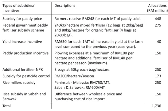
Table 1. Farmer’s expenditure and subsidies on agrochemicals (rice sector), 2009
Agrochemicals Own expenditure Value of subsidies Subsidies (ad valorem) per hectare (RM) per hectare (RM) Column 3/(Column 2 + Column 3)
Fertiliser 99.6 62.2 38.4%
Chemical 240.7 655.8 73.2%
Source: Universiti Kebangsaan Malaysia (2009).
2. Overview of Malaysian Rice Sector
Malaysia’s rice production, consumption and imports show an increasing trend over the four recent decades. Still, the production of rice is only sufficient to meet on average about 73 percent (ranging from 58.8 percent to 90.4 percent) of domestic needs, with the remaining 27 percent being imported mainly from Thailand and Vietnam (calculated based on United States Department of Agriculture [USDA], 2012).
All aspects of the rice trade are controlled by Padiberas National Berhad (BERNAS), a government cooperation. Monopoly power is given to BERNAS in rice trading in order to ensure a fair price for consumers (World Trade Organization [WTO], 2006).
Although the existence of BERNAS has trade-distorting effects, the government also imposes high import duties on rice. The import duties for rice imports are 40 percent under the Agreement on Agriculture (AoA) of the WTO and 20 percent under the Common Effective Preferential Tariff Agreement (CEPT) of the ASEAN Free Trade Area (AFTA).
As shown in Table 2, over 1.63 million tons of rice were produced in 2011 as compared to only 0.75 million tons in the 1960s. Over the same period, the con- sumption and import of rice also increased from 1.2 million and 0.45 million to 2.77 and 1.13 million tons, respectively, while the harvested area increased only from 528 to 670 thousand hectares. The area harvested has been rising slowly until the 1980s. Since then it has been stable between 662 to 670 thousand hectares.
The relation between production, consumption and imports in the rice sector has been affected mainly by policy interventions which aimed to regulate and protect the industry. Tables 3 and 4 summarise the comprehensive market interventions in various forms.
Table 2. Rice production, consumption, imports and harvested area (1960-2011)
Year Production Domestic Imports Exports Harvested
consumption area
(1000 MT) (1000 MT) (1000 MT) (1000 MT) (1000 HA)
1960 749 1,200 451 0 528
1970 1,091 1,345 356 0 697
1980 1,318 1,500 167 0 696
1990 1,302 1,490 298 0 662
2000 1,410 1,946 596 0 665
2005 1,440 2,150 751 0 660
2010 1,610 2,665 1,040 1 667
2011 1,630 2,770 1,130 1 670
Note: MT and HA refers to metric tons and hectares, respectively.
Source: USDA (2012).
Table 3. Subsidies and incentives in rice sector, 2009
Types of subsidies/ Descriptions Allocations
incentives (RM million)
Subsidy for paddy price Farmers receive RM248 for each MT of paddy sold. 448 Federal government paddy 240kg/hectare mixed fertiliser (12 bags at 20kg/bag) 275 fertiliser subsidy scheme and 80kg/hectare for organic fertiliser (4 bags at
20kg/bag).
Yield increase incentive RM650 for each 1MT of increase in yield at the farm 40 level compared to the previous year (base year).
Paddy production incentive Plowing expenses at a maximum of RM100 per 150 hectare and additional fertiliser of RM140 per
hectare per season (maximum).
Additional fertiliser NPK 3 bags at 50kg each bag/hectare. 250
Subsidy for pesticide control RM200/hectare/season. 173
Rice millers subsidy Peninsular Malaysia: RM750/MT. 250
Sabah & Sarawak: RM600/MT.
Rice subsidy in Sabah and Difference between wholesale price and 150 Sarawak purchasing cost of rice import.
Total 1,736
Source: Ministry of Agriculture and Agro-Based Industry (2010).
Table 4. Paddy and rice programmes in the National Food Security Policy
Programme Description
Availability Irrigation infrastructure and Develop new water source and increase irrigation drainage development infrastructure and drainage density to the optimum
level of 50m/ha.
Irrigation infrastructure and Maintain paddy field area both in granary area or drainage maintenance non-granary area.
Land levelling Implement land levelling activity to improve the efficiency of good agricultural practices. Rate of land levelling is as much as RM1,500/ha.
Lime application Supply lime to improve soil fertility. The aid is RM850/ha.
Farm mechanisation Increase number of machinery in rice cultivation.
Beras Nasional Subsidised 15 percent broken rice and retailed at RM1.80/kg throughout Malaysia.
Accessibility Beras Nasional Subsidised 15 percent broken rice and retailed at RM1.80/kg throughout Malaysia.
Utilisation Research and development Promote new methods of paddy cultivation to
increase productivity.
Stability Stockpiling Increase stockpile level of 92,000MT to 239,000MT.
Source: Tey (2010).
3. Literature Review
Wide numbers of literature exist on the assessments of agricultural policies. The most common approaches are econometric and market equilibrium models including partial equilibrium (PE) and computable general equilibrium (CGE) models.
The basic characteristic of econometric models is the use of historical or cross- sectional data to estimate the underlying model’s parameters through a variety of estimation techniques. Pollitt, Chewpreecha and Summerton (2007) discussed that econometric models are often very resource-intensive and for this reason alone, their use tends to be somewhat limited. Another criticism of econometric models is that they are subject to the Lucas Critique. This states that it is simplicity to predict the effect of a policy experiment based on the relationships estimated from historical data. Market equilibrium models, on the other hand, often require just a single year data for model calibration. They are also not generally subject to the Lucas Critique as the outcome tends to be shaped by the underlying microeconomic behavioural foundations.
While PE models in contrast to the CGE model do not cover the whole economy, but only selected sectors, they typically describe these sectors with detail of supply and demand, factor markets and price linkages. Owing to the emphasis on a single, or few sectors, they can provide a focussed and tractable analysis of how a limited number of variables is affected by policy changes or restrictions. A downside of the PE approach can be that analyses of sectors with a high share of GDP (like agriculture as a whole in poor countries) might underestimate macroeconomic effects of sectoral policies. This problem, however, does not apply for paddy rice in Malaysia which accounts for less than 1 percent of national GDP.
This paper develops a comparative static PE model for the Malaysian rice sector which explicitly links factor markets, related output, domestic demand and trade.
The model is then used to examine the impact of the reduction in agrochemical input subsidies and a shift toward the use of organic inputs. The developed model is based on a so-called market (equilibrium) displacement model as introduced by Muth (1964) and Floyd (1965) and popularised in agricultural economics by Gardner (1987) in his textbook. Hertel (1989) used the idea to develop a single country PE model with an explicit treatment of factor markets. Gunter, Jeong and White (1996) extended Hertel’s framework to a multi-country model and since then there are various applications of the models and their extensions (see, for example, Alston & James, 2002; Ciaian &
Kancs, 2009; Ciaian & Swinnen, 2006; Jamal, 2003; Salhofer, 1996; among others). Jafari and Jamal (2015; 2016) also constructed a multi-commodity model which is based on Hertel’s single sector model and applied the model to the Malaysian agricultural sector to appraise the impact of trade and biofuel policies in the oil palm sector.
While there exist several studies on the impact of trade and output policies in the Malaysian rice sector, the literature on the impact of input subsidy interventions and shifting from agrochemical to organic inputs is limited. Perhaps the closest study to our analysis is the study by Umar, Abdullah, Shamsudin and Mohamed (2016) analysing the welfare and market impacts of fertiliser subsidy withdrawal in the Malaysian rice sector using econometric techniques. Their results suggest that a removal of fertiliser subsidies would lead to a loss of producer surplus (RM839 million) and savings in
government expenditure (RM183 million), and thus a net increase of RM655 million in social welfare. Further, as a result of the subsidy removal, imports are claimed to have increased by 19 percent, while rice production is projected to decrease by 10 percent.
The study, however, only focused on producers and did not simulate market outcomes.
Hence, we still see sufficient scope to analyse the impact of the reduction in the use of agrochemicals through various policy options using a partial equilibrium model, where substitution possibilities between inputs are considered in a factor market module, and where output and trade markets are explicitly considered.
4. Methodology and Data
4.1 The Partial Equilibrium Framework
The Malaysian rice sector model is comprised by functions that represent supply (production and imports) of, and demand (consumption and exports) for rice. On the supply side, a representative firm combines multiple input factors including land, labour, agrochemicals and capital to produce the output. The supply of each of these inputs is dependent on the return to the factor and the availability of resources controlled by the input factor supply elasticities. Input demands are derived demands under the condition of locally constant returns to scale. The substitution between inputs is permitted through cross price elasticities. The factor market clearing conditions ensure that there is no excess demand/supply of inputs. On the demand side, the market consumption is the sum of domestically produced and imported rice. Output market clearing conditions ensure that output supply and demands are equal. Since all modules of the model (factor markets, output and demand markets, and trade) are interlinked, any policy shocks or exogenous changes affecting the input market have consequences on the use of inputs, demand and supply quantity and price of outputs, and imports. Finally, welfare functions are incorporated to capture consumer, producer and taxpayer’s surplus.
In order to provide these linkages in a mathematical framework, we construct the model in a way that captures the following linkages: (i) linkages between environmental policy, and input use and returns, (ii) the underlying agricultural production function which links the primary factors of production to output supply, (iii) the underlying welfare function which links the welfare of various interest groups (consumers, producers and taxpayers) to the return and use of the primary factors of production and the quantity and price of output produced. The algebraic setup and the theoretical foundations of these linkages are subsequently discussed.
Table 5 describes the model in its general form while its differentiated form which is actually used in the simulation exercise and the detailed mathematical procedure based on which the differentiated form arrives is discussed in Appendix A. The differentiated form is a comparative static long run model based on total differentiation of a system of equations but manipulated in a way to have elasticities and shares rather than slopes as arguments.
In this framework, Q and P refer to demand quantity and price, respectively.
Subscript y refers to output, while i and j refer to input quantities or prices. Superscript M refers to the market quantities and domestic market prices. Thus, denotes market PyM
price of output y. Superscript DD refers to demand for domestically produced output, and MD refers to import demand so that and refer to the quantity of demand for domestically produced goods and import demand, respectively. Superscript F refers to the farm (rice in our analysis) sector. Thus, is quantity of input demand by farm sector in response to changes in prices of input ( ), and farm output supply ( ).
Further, superscript ROW refers to import supply from the rest of the world, while W refers to world prices. The difference symbol (∆) shows the changes in consumer surplus (cs), producer surplus (ps) and taxpayer’s surplus (ts) from their initial values to the values after policy shock denoted in the prime symbol (′).
4.1.1 Commodity Demand Module
Both local and imported rice in Malaysia are consumed in the domestic market, and there is no export of this product from the country. Accordingly, the first equation in Table 5 addresses the market demand ( ) as sum of demand for domestically produced output ( ) and import demand ( ). Further, assuming that consumers have homothetic preferences, the next two equations define and as functions of market demand price , and world price ( ). By total differentiation of demand equations and manipulating them to obtain the elasticities and market shares, the equations in percentage form are defined as A1 through A3 in Appendix A.
Table 5. Long run partial equilibrium model of rice sector (general form)
1 Market demand
2 Domestic demand
3 Import demand
4 Derived factor demand
5 Zero profit condition
6 Factor supply
7 Import supply
8 Ad valorem input policy
9 Ad valorem output policy
10 Input market clearing conditions
11 Output market clearing condition (Foreign
market)
12 Output market clearing condition (Domestic
market)
13 Changes in consumer surplus
14 Changes in producer surplus
15-1 Changes in taxpayers surplus (when input
tax/subsidy policy is implemented)
15-2 Changes in taxpayers surplus (when input
demand shift is implemented)
QyDD QyMD
QFj
PiF QyF
∆ = ′ −TS QyF Q ∗ + ′ −t Q Q ∗s
yF
y jF
jF
( ) ( ) j
∆ = ′ −TS QjF Q ∗ + ′ −s P P ∗Q
Fj
j jF
jF jF
( ) ( )
∆ =CS CS CS− ′
∆ =PS PS PS− ′ QyF Q
yDD
= QyROW Q
yMD
= QjS Q
jF
= PyM t P
y yF
= PiM s P
j jF
=
QyROW Q P
yROW yW
= ( ) QjS=Q PjS( )jM PyF P P P
yF iF
nF
= ( , , ) QFj Q P P Q
jF iF
nF yF
= ( , , , ) QyDD Q P
yDD yM
= ( ) QyMD Q P P
yMD yM
yMD
= ( , ) QyM Q Q
yDD yMD
= +
QyM
QyD QyMD
QyD QyMD
PyMD
PyM
4.1.2 Derived Demand for Inputs
Conditional factor demands for inputs can be derived under certain assumptions of cost minimisation and perfect competition. Assuming that cost function is mathematically well-behaved and twice differentiable so that first and second order conditions are valid, one can derive conditional factor demand functions using Shephard’s lemma and the Envelope theorem. Equation 4 refers to the general specification of factor demand function. Superscript F refers to the farm sector (i.e. rice sector) such that represents the input quantity demanded by farm sector in response to changes in input prices ( ) and output supply ( ). Translating this equation into the differentiated forms and extending it to capture for the impact of a shift in input demand schedules results in A4 (Appendix A). Shifts in input demand schedules are especially incorporated into the model to capture the impact of the shift in demand for agrochemicals reflecting a campaign targeting the environmental quality degradation, highlighting a critical, yet sensitive contemporary development policy issue in Malaysia.
4.1.3 Zero Profit Conditions
Under the assumption of perfect competition and constant return to scale, firm’s profit, in the long run, is equal to zero. Equation 5 refers to zero profit condition when the firms’ output price ( ) is equal to a unit cost function defined as general function of input prices ( ). This equation in differentiated form appears as A5.
4.1.4 Factor Supply and the Supply from ROW Function
Supply of jth input ( ) in response to changes in market price of inputs ( ) is defined in Equation 6. The next equation depicts the supply from Rest of the World (ROW) ( ) as function of World prices ( ). Note the assumption that rice is supplied from the ROW to Malaysia at an exogenously determined price under the ‘small country assumption’ where the world market price is fixed. The supply functions in differentiated forms are defined as A6 and A7.
4.1.5 Ad Valorem Equivalent (AVE) Policies
Input and output policies in the model are denoted in ad valorem forms. Equation 8 refers to input subsidy (s ˃ 0) that lower the cost which farmers must pay relative to the non-rice opportunity cost of input. Next equation denotes domestic output subsidy ( ). Since there will be no changes in output policies in our analysis, changes in supply and market prices are equal. AVE policies in percentage changes form are defined as A8 and A9.
4.1.6 Output and Input Clearing Conditions
These conditions require that prices must adjust to equilibrate domestic supply ( ) and demand for domestically produced output ( ); import supply from the ROW ( ) and import demand ( ); and input supply ( ) and input demand ( ). These conditions are reflected in equations 10 through 12 and their differentiated forms appear in A10 through A12.
QjF
PjF QyF
PjF PyF
QjS PjM
QyROW PyW
ty<0
QyF QyDD
QyROW QyMD QiS QFi
4.1.7 Welfare Functions
In this study, in order to show the interaction between policy maker’s behaviour and the welfare of various interest groups including consumer, producer and taxpayers, the welfare function is incorporated. The incorporation for welfare impacts is due to Paarlberg and Abott (1986). Change in national welfare is the sum of changes in the welfare of various interest groups for whom their welfare changes due to policy changes are measured.
Figure 1 depicts the equilibrium situation in the output market. The initial equi- librium is E where the prevailing market price and quantity are and , respectively.
Reduction in input subsidies shifts the output supply curve upward from to and as a result the new equilibrium is E´. Accordingly, a change in consumer surplus (Equation 13) is equal to the area , which is calculated as . Knowing that and substituting them into the CS equation results in,
(13) Similarly, as illustrated in Figure 2, the changes in producer surplus (Equation 14) following a reduction in input subsidies is equal to the area , measured as,
(14) PyM QyM
QyF Q′yF
P E EPyM yM
′ ∆ =CS ∗ ′ ′ +P E EPyM ∗ ′P P
yM yD
yD
0 5. ( )
P E EPy′ ′F yF
𝑃𝑃𝑦𝑦𝑀𝑀
𝑄𝑄𝑦𝑦𝑀𝑀 𝑄𝑄𝑦𝑦𝑀𝑀
𝑸𝑸𝒚𝒚𝑭𝑭
𝑄𝑄′𝑦𝑦𝑀𝑀 𝑃𝑃′𝑦𝑦𝑀𝑀
E
𝑸𝑸′𝒚𝒚𝑭𝑭
E′
𝑃𝑃𝑦𝑦𝑀𝑀 H
Figure 1. Consumer welfare impact of reduction in agrochemical subsidies
ˆ ˆ
( ); ;
D M M M M M M M M D D
y y y y y y y y y y y
P E Q Q Q Q EP Q P P P P
1[ ( ˆ ) ] ˆ ˆ (1 0.5 )ˆ
2
M M M M D D D M D M
y y y y y y y y y y
CS Q Q Q Q P P P Q P Q
1[ ( ˆ ) ] ˆ ˆ (1 0.5 )ˆ
2
S S S S S S S S S S
y y y y y y y y y y
CS NQ Q Q Q P P P Q P Q
Total tax payment is the sum of output and input taxes. Changes in total output tax payment is equal to changes in output supply ( ) multiplied with benchmark output tax (ty). Further, the change in the amount of tax paid by the producer on its use of input depends on the type of policy implemented. When a shift in demand schedule is assumed, changes in taxpayer welfare is equal to the change in demand for inputs ( ) times the benchmark input tax (ti) . However, when the change in input subsidy is practised, the change in taxpayer welfare is equal to the area (Figure 3). Equations 15-1 and 15-2 reflect the changes in taxpayer’s surplus.
It should be noted that, given the nature of partial equilibrium model, a welfare change of a policy that has impacts beyond the rice market is disregarded. For example, the funds not spent in direct agrochemical subsidies will presumably be employed somewhere else in the economy and might generate a ‘double-dividend’
type of effect.
Equations A1 through A15 show the structure of the PE model in reduced form where all prices and quantities and welfare are treated as endogenous variables while the policy variables and the parameters of the model are exogenous in the model. Note that the equations in the model have been linearized and hence the magnitude of impacts for greater policy perturbation will simply be linear multiples of the impacts deliberated in this study. For instance, a 30 percent reduction in the use of agrochemical subsidies would show as three times the impact of a 10 percent reduction. However, since the model is linear, it can only be limited to appraising small policy perturbations, perhaps to less than 30 percent.
Figure 2. Producer welfare impact of reduction in agrochemical subsidies
𝑃𝑃𝑦𝑦𝐹𝐹
𝑄𝑄𝑦𝑦𝑆𝑆 𝑄𝑄𝑦𝑦𝑆𝑆
𝑸𝑸𝒚𝒚𝑴𝑴
𝑸𝑸𝒚𝒚𝑭𝑭
𝑄𝑄′𝑦𝑦𝑆𝑆
E
𝑸𝑸′𝒚𝒚𝑭𝑭
E′
𝑃𝑃′𝑦𝑦𝐹𝐹
𝑃𝑃𝑦𝑦𝐹𝐹
R H
Q′ −yS Q
yS
Q′ −iF Q
Fi
P E HPi′ ′F iF
4.2 Baseline Data
Before any simulation is performed, the baseline parameters or coefficients for the endogenous variables must be established. Likewise many partial and general equilibrium models include a large number of parameters, where some of the parameters of the present model are obtained, calibrated or assumed (Salhofer, 2000).
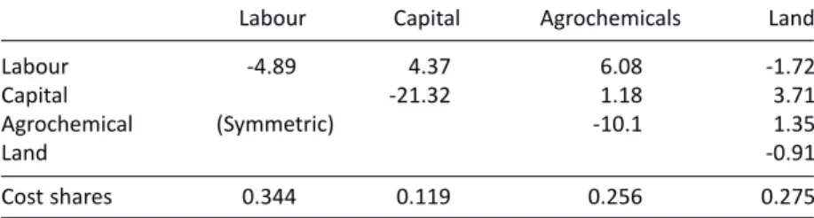
Table 6 shows the Allen elasticities of substitution between inputs (σij) and factor cost shares (cj). The Allen elasticities shows the substitution possibilities between various types of inputs in response to changes in own input price or price of other inputs. The factor cost shares show the share of each input in the unit cost function.
The input supply elasticities (vj) in Malaysia, as defined in the model, are not directly available from the literature, but have to be deduced from the review of studies of this kind. Salhofer (2000) reviewed microeconomic studies on the farm level primary factor supplies and recommended to use the mean value of maximum and minimum point elasticities found in literature as a benchmark data. Hence, the value of input supply elasticities in this study follows from Salhofer (2000) (see Table 7). Further, as shown in Table 8, the benchmark value for the prices of inputs used in rice sector ( ) are calculated based on subtracting the subsidies received by firms from the market prices ( ). The price and the quantity of rice produced and consumed in the domestic market are shown in Table 9.
The value of -0.3 for domestic rice and import demand elasticity ( ) is taken from the Food and Agricultural Policy Research Institute (FAPRI) elasticities database.
Figure 3. Producer welfare impact of reduction in agrochemical subsidies
𝑃𝑃𝑖𝑖𝐹𝐹
𝑄𝑄𝑖𝑖𝐹𝐹, 𝑄𝑄𝑖𝑖𝑆𝑆 𝑄𝑄𝑖𝑖𝐹𝐹
𝑸𝑸𝒊𝒊𝑭𝑭
𝑸𝑸𝒊𝒊𝑺𝑺
𝑄𝑄
′
𝑖𝑖𝐹𝐹 𝑃𝑃′
𝑖𝑖𝐹𝐹E
𝑸𝑸
′
𝒊𝒊𝑺𝑺E
′
𝑃𝑃𝑖𝑖𝐹𝐹 H
PiF
PiM
εyDD,εyMD
It is assumed that the supply elasticity of import with respect to import price (0.3) is equal in quantum with cross price import elasticity ( ). The value of import and domestic share parameters (0.29, 0.71) are calculated based on United States Department of Agriculture (USDA) (2011).
It is important to note that although changes in the baseline coefficients of the endogenous variables in the model may lead to changes in the magnitude of exogenous variables, our sensitivity analysis1 reveals that the direction and relative order of impacts of the result would still be reliable, provided that the meaningful sign is given to the substitution or complementary possibilities.
Table 6. Allen elasticities of substitution between inputs in rice cultivation
Labour Capital Agrochemicals Land
Labour -4.89 4.37 6.08 -1.72
Capital -21.32 1.18 3.71
Agrochemical (Symmetric) -10.1 1.35
Land -0.91
Cost shares 0.344 0.119 0.256 0.275
Source: Naziruddin Abdullah (2002).
Table 7. Input supply elasticities, and domestic and import demand shares
Land supply elasticity 0.3
Labour supply elasticity 0.55
Agrochemical supply elasticity 2
Capital supply elasticity 2
Source: Salhofer (2000).
Table 8. Market price and firm demand price (2009) (RM million) Market price Firm demand price
Fertiliser 656 473
Chemical 9,059 4,854
Source See Appendix B Market price x (1- subsidy rate) Table 9. Price, production, and consumption of rice in Malaysia (2009)
Variable Value Source
Consumer price ( ) (RM values per ton) 1,923
Producer price ( ) (RM values per ton) 998 See Appendix B Rice market demand ( ) (1000 ton) 3,686
Rice domestic production ( ) (1000 ton) 2,510 USDA (2011)
1 The sensitivity analyses are not included in the paper to save space.
PyM
PyF
QMy QFy
ψ yMD
}
5. Results and Discussions
The constructed model is employed to appraise the effects of a reduction in input subsidies and shifts in input demand schedule due to some exogenous factors which represent the government’s attempts to reduce the use of agrochemicals in the context of GAP. This paper first considers a 10 percent reduction in agrochemical subsidies in the Malaysian rice sector. The result is compared with that of a 10 per- cent and 2 percent unilateral downward shift in agrochemical demand schedule.
Technically, a unilateral 10 percent shift in agrochemical demand schedule represents the government’s attempts to reduce the use of agrochemicals in the context of GAP while a unilateral 2 percent downward shift reflect the government’s attempt to encourage the use of environmentally friendly inputs. Simulation results, i.e. effects of a reduction in agrochemical subsidies and the parameter shift (policy changes) on the endogenous variables are listed in Tables 10 and 11 for all scenarios. It shall be noted here that the major focus of this type of appraisals is on the direction and the relative order of impacts.
The results generally show an expected long-run impact among the endogenous variables representing environmental quality (agrochemical uses and land demand), food security (paddy output) and the welfare of various interest groups. As can be seen in Tables 10 and 11, a reduction in agrochemical subsidies and a downfall shift in agrochemical demand schedules lower the demand for agrochemicals, thus reducing the supply of paddy, and hence decrease the welfare of both producers and consumers and decrease government expenditure on providing agrochemical subsidies and consequently results in less national welfare when there is a reduction in agrochemical subsidies and increased national welfare when there is a downfall shift in agrochemical demand schedules.
In the first scenario, i.e. a 10 percent reduction in agrochemical subsidies leads to a fall in the demand for agrochemicals and land demand by 7.36 percent and 0.39 percent, respectively, while the number of employment and use of capital related inputs, which are being used as primary inputs for paddy, will increase. However, a reduction in agrochemical subsidies provokes an increase in paddy prices (2.81 percent), reduces the demand for and supply of paddy, and consequently weakens the food security level (-0.84 percent). Additionally, as shown in Table 11, a reduction in agrochemical subsidies reduces the welfare of both consumers and producers, while it increases the welfare of taxpayers. It is estimated that the increase in taxpayer’s welfare will not be able to compensate for the reduction in consumer and producer surpluses.
Consequently, given the same weight of importance to the various interest groups, the national welfare is expected to decrease.
On the other hand, the results from the second scenario, i.e. simultaneous down- ward demand shifts of 10 percent in agrochemicals has comparable impacts to that of a 10 percent reduction in chemical and pesticides subsidies. However, as a result of the downfall shift in agrochemical demand schedules, national welfare will increase by a value of about RM165.9 million. Additionally, the direction and order of changes in other endogenous variables are almost the same (Tables 10 and 11). While the direction of the impact of fall in agrochemical demand being used in the production of Malaysian
paddy on variables of interest is similar in both scenarios, the quantum of impacts is substantially larger in the first scenario.
For instance, while a reduction in agrochemical subsidies will reduce agrochemical and land demand by 7.63 percent and 0.39 percent respectively, and hence, paddy production by 0.84 percent, the agrochemical use restriction scenario will result in a more pronounced drop in agrochemical and land demand by 6.79 percent and 0.04 percent respectively, and thereby reducing the paddy output by 0.31 percent. The Table 10. Effects (% changes) of alternative policies on endogenous variables
Policy shocks
Variable 10% reduction 10% downfall shift 2% downfall shift
in agrochemical in agrochemical in agrochemical subsidies demand schedule demand schedule Output market
Market demand for paddy -0.36 -0.13 -0.03
Domestic supply for paddy -0.84 -0.31 -0.06
Import demand for paddy 0.84 0.31 0.06
Domestic price of paddy 2.81 1.02 0.20
Factor market
Land demand -0.39 -0.04 -0.01
Labour demand 2.56 2.74 0.55
Agrochemical demand -7.63 -6.79 -1.36
Capital demand 2.67 3.95 0.79
Price of demand for land -1.94 -0.21 -0.04
Price of demand for labour 4.66 4.97 0.99
Price of demand for agrochemical 6.19 -3.39 -0.68
Price of demand for capital 1.33 1.97 0.39
Table 11. Effects (absolute changes) of alternative policies on welfare (RM million) Policy shocks
Variable 10% reduction 10% downfall shift 2% downfall shift
in agrochemical in agrochemical in agrochemical subsidies demand schedule demand schedule
ΔCS Changes in consumer surplus -199.6 -72.3 -14.5
ΔPS Changes in producer surplus -70.7 -25.6 -5.1
ΔTS Changes in taxpayers surplus 119.3 263.8 275.3
Changes in national welfare -151.0 165.9 255.8
QMy QFy
QMDy
PyM
QLandF
QLabF
QCheF
QCapF PLandF
PLabF
PCheF
PCapF
impact of agrochemical subsidies reduction is also more profound on consumer and producer surplus and is less profound on taxpayer’s welfare in Malaysia. Such results are naturally expected as the higher reduction in agrochemical demand will not be adequately offset by increases in the use of other inputs.
However, the effect of a 2 percent downfall shift in agrochemicals which is assumed to have comparable impacts with government attempts toward encouraging environmental friendly inputs would result in more desirable impacts in terms of consumer and producer surplus, food security, environmental quality, welfare of various interest groups as well as overall national welfare.
6. Conclusion and Policy Implications
Agricultural policies were designed to shape the Malaysian paddy subsector through commodity and input price changes and consequently have implications for the welfare of various interest groups, input and output markets as well as trade. This study considers three different scenarios to examine the impact of a reduction in the use of agrochemicals including chemical based fertilisers and pesticides on the variables of interest including agricultural land use, agrochemicals, paddy output and, the welfare of various interest groups including consumers, producers and taxpayers in Malaysia.
The first scenario examines the impact of a 10 percent reduction in agrochemical subsidies in the rice sector, the second scenario considers the simultaneous impact of a unilateral 10 percent reduction in the demand schedule for chemical based fertilisers and pesticides being used in Malaysian rice cultivation, while the third scenario appraise the impact of encouraging the use of environmental friendly inputs.
Results from the model indicate that a reduction in agrochemical subsidies is expected to demonstrate considerable effects on the quality of the environment while decreasing national welfare and weaken food security. Further simulation denotes a reduction of 10 percent in demand for agrochemicals has comparable impacts to that of a 10 percent reduction in chemical and pesticide subsidies except that it increases the national welfare. One may think that any fall in the use of agrochemicals would lead to serious national concerns as Malaysia would still aim at sustaining her food sufficiency level and improve the welfare of all consumers and producers. Overall, the result shows that although the environmental policies in forms of either a reduction in agrochemical subsidies or a downfall in the supply of agrochemicals have a negative effect on the self- sufficiency level, the use of factor demands as a result of output contraction decreases.
Therefore, less agricultural land is demanded and a huge amount of chemical and fertilisers moves away from the rice sector.
However, should the Malaysian government wish to encourage the use of environmental-friendly inputs which can compensate for a fall in reduction of agro- chemical inputs, the impacts to Malaysian rice subsector, including environment and welfare are expected to be considerable, while food safety will be affected far less than that of reduction in agrochemical subsidies or restriction on use of inputs when the use of organic inputs are not encouraged.
Overall results imply that encouraging the use of organic inputs which are seen as important for the sustainable development and management of natural resources
might have a more desirable impact on the variables of interest relative to reducing agrochemicals either through subsidy reduction or input restriction.
The growing concern to rice producers in Malaysia is to find out the best policy option which improves the quality of environment while increasing or at least not decreasing the food security level as well as national welfare. Future studies may employ an endogenous policy formation model to secure the benefits of policies in favour of particular interest group based on some strategic or national interest such as social and environmental stability, or national food security needs. The environmental benefits from a reduced use of chemical fertilisers and pesticides are not modelled in this study. One would expect that environmental benefits from reduced agrochemical use would include improvements in water quality with direct implications for eco- systems and human health. Further, although environmental benefits of removing the subsidy or reducing agrochemical use are discussed in the paper, it does not measure or incorporate them into their welfare accounting. These environmental benefits would presumably benefit consumers and producers. Future studies are warranted to take into account such modelling issues.
References
Agriquest Sdn Bhd, Malaysia. (2009). Malaysian agricultural directory and index 2009/2010. Kuala Lumpur: Author.
Alston, J.M., & James J.S. (2002). The incidence of agricultural policy. In B.L. Gardner and G.C.
Rausser (Eds.), Handbook of agricultural economics (pp. 1689-1749). Amsterdam: Elsevier.
Azmi Mat Akhir, Roziah Omar, & Hamidin Abd Hamid. (2009). Food security – A national responsibility of regional concern: Malaysia’s case. Paper presented at a Conference on Food Security and Sustainable Development, Rome, 11-13 November.
Ciaian, P., & Kancs, d’A. (2009). The capitalization of area payments into farmland rents: Theory and evidence from the new EU member states (EERI Research Paper Series No. 04/2009).
Brussels: Economics and Econometrics Research Institute.
Ciaian, P., & Swinnen, J.F.M. (2006). Land market imperfections and agricultural policy impacts in the new EU member states: A partial equilibrium analysis. American Journal of Agricultural Economics, 88(4), 799-815. https://doi.org/10.1111/j.1467-8276.2006.00899.x
Fatimah Mohamed Arshad, Nik Mustapha Raja Abdullah, Bisant Kaur, & Amin Mahir Abdullah (Eds). (2007). 50 years of Malaysian agriculture: Transformational issues, challenges and direction. Serdang: Universiti Putra Malaysia Press.
Food and Agricultural Policy Research Institute (FAPRI). (n.d.). Elasticities database. Retrieved from http://www.fapri.iastate.edu/tools/elasticity.aspx
Food and Agriculture Organization (FAO). (n.d.). FAO statistic database. Retrieved from http://
faostat.fao.org/site/575/default.aspx#ancor
Floyd, J.E. (1965). The effects of farm price supports on the returns to land and labor in agricul- ture. Journal of Political Economy, 73(2), 148-158. http://dx.doi.org/10.1086/259003 Gardner, B.L. (1987). The economics of agricultural policies. New York: McGraw-Hill.
Gunter, L.F., Jeong, K.H., & White, F.C. (1996). Multiple policy goals in a trade model with explicit factor markets. American Journal of Agricultural Economics, 78(2), 313-330. https://doi.
org/10.2307/1243705
Hertel, T.W. (1989). Negotiating reductions in agricultural support: Implications of technology and factor mobility. American Journal of Agricultural Economics, 71(3), 559-73. https://doi.
org/10.2307/1242012
International Monetary Fund (IMF). (2012). IMF data. Retrieved from http://www.imf.org/en/
Data.
Jafari, Y., & Jamal Othman. (2015). A comparative static, partial equilibrium, multi-commodity model for Malaysian agriculture. Malaysian Journal of Economic Studies, 52(2), 205-226.
Jafari, Y., & Jamal Othman. (2016). Impact of biofuel development on Malaysian agriculture: A comparative statics, multicommodity, multistage production, partial equilibrium approach.
Food and Energy Security, 5(3), 192-202. doi: 10.1002/fes3.84
Jamal Othman. (2003). Linking agricultural trade, land demand, and environmental externalities:
Case of oil palm in Southeast Asia. ASEAN Economic Bulletin, 20(3), 244-255.
Knoema. (2013). Fertilizer use by crop, 2013. Retrieved from https://knoema.com/IFAFUBC2013/
fertilizer-use-by-crop-2013?country=1000100-malaysia
Ministry of Agriculture and Agro-Based Industry. (2010). Senarai bantuan, subsidi dan insentif industri padi dan beras, tahun 2009 (Bahasa Malaysia). Retrieved from http://www.moa.gov.
my/web/guest/insentif_padi_n_beras
Mohamed Ali Sabri. (2009). Evolution of fertilizer use by crops in Malaysia: Recent trends and prospects. Paper presented at the IFA Crossroads Asia-Pacific 2009 Conference, Kota Kinabalu, Malaysia, 8-10 December.
Mohamed, Z., Terano, R., Shamsudin, M.N., Abd Latif, I. (2016). Paddy farmers’ sustainability practices in granary areas in Malaysia. Resources, 5(2), 17. doi:10.3390/resources5020017 Mohammad Anvar, & Basri Abdul Talib. (2008). An assessment of support on paddy farmers in
Malaysia. Bangi: Universiti Kebangsaan Malaysia Project.
Muth, R.F. (1964). The derived demand curve fora productive factor and the industry supply curve. Oxford Economic Papers, 16(2), 235-261.
Naziruddin Abdullah. (2002). Measurement of technological change biases and factor substi- tutions for Malaysian rice farming. IIUM Journal of Economics and Management, 10(1), 1-20.
Paarlberg, P.L., & Abott, P.C. (1986). Oligopolistic behavior by public agencies in international trade: The world wheat market. American Journal of Agricultural Economics, 68(3), 528-542.
https://doi.org/10.2307/1241538
Pollitt, H., Chewpreecha, U., & Summerton, P. (2007). E3ME: An energy–environment–economy model for Europe: A technical description. Retrieved from http://www.petre.org.uk/pdf/
E3ME_Technical_Description_v4.2.pdf
Salhofer, K. (1996). Efficient income redistribution for a small country using optimal combined instruments. Agricultural Economics, 13(3), 191-199.
Salhofer, K. (2000). Elasticities of substitution and factor supply elasticities in European agricul- ture: A review of past studies. In Organisation for Economic Co-operation and Development (2001), Markets Effects of Crop Support Measures (pp. 89-110). Paris: OECD Publishing.
Tey, Y.S. (2010). Malaysia’s strategic food security approach. International Food Research Journal 17(3), 501-507.
Umar, H.S., Abdullah, A.M., Shamsudin, M.N., Mohamed, Z.A. (2016). Implication of fertiliser subsidy withdrawal on societal welfare, rice output and imports in Malaysia’s rice sector.
Pertanika Journal of Social Sciences & Humanities, 24(2), 777-794.
United States Department of Agriculture (USDA). (2011). Retrieved from http://www.fas.usda.
gov/psdonline
United States Department of Agriculture (USDA). (2012). Production, Supply and Distribution Database (PSD Online). Retrieved from https://apps.fas.usda.gov/psdonline/
Universiti Kebangsaan Malaysia (UKM). (2009). Project on Development of Food Balance Sheet System for Malaysia, Ministry of Agriculture and Agro-based Industries, 2008-2009.
World Trade Organization (WTO). (2006). Trade policy review: Trade policies by sector. Retrieved from https://www.wto.org/english/tratop_e/tpr_e/tpr_e.htm
Appendices
Appendix A: Single Commodity Partial Equilibrium Model of the Malaysian Rice Sector Definition of parameters and variables of the model
Table A1 provides the definitions of parameters and variables of the model. Note that the hat notation symbolises percentage changes in variables (e.g. ), while the notation d refers to absolute changes in variables.
Q dQ
y Q
M yM
yM
=
Table A1. Definitions of variables for the partial equilibrium model Endogenous variables
Market demand, demand for domestically produced good, and import demand for y, respectively.
Domestic farm supply, and the Rest of the World (ROW) supply of y, respectively.
Farm, and market, and the world price for y, respectively.
Farm factor supply and demand, respectively.
Market price and farm sector price for inputs, respectively.
CS, PS, TS Consumer, producers and taxpayer surpluses, respectively.
Parameters
The elasticity of demand for domestically produced y and imported y with their associated prices, respectively.
Elasticity of import demand with respect to changes in domestic prices.
Import supply elasticity of y.
Allen substitution elasticity between input i and j.
The cost share of jth input with respect to total cost of producing y.
Supply elasticity of jth input
Shares of domestic demand and import demand of the total market demand, respectively.
Exogenous variables (policy shocks) Input subsidy on use of j.
Output subsidy.
Shift in demand schedules for jth input.
Q Q QyM yDD
yMD
, , Q QFy
yROW
,
Derivation of the model in its differentiated form
This section discusses the mathematical derivation of the model in differentiated form.
The total differential of (1) leads to:
P P PyF
yM yW
, , Q QiS
iF
, P PMj
j
, F
εyDD,εMDy ψyMD εyROW σij Cj
vj
αyDD,αyMD
sj ty
UFj
dQyM dQ dQ
yDD yMD
= +