Introduction
Context and motivation
In this thesis we are interested in the low-energy properties of the systems we study. Some of the most successful algorithms in terms of accuracy, efficiency and flexibility (to study a variety of different models) are based on tensor networks.
Tensor networks
The PEPS network structure is designed to satisfy the entanglement zone law for 2D ground states [ 31 , 32 ]. A related consequence is that the PEPS lacks a canonical form equivalent to that of the MSHP.
Summary of research
By convention from the previous sections, (1,1) corresponds to the lower left corner and (𝐿𝑥, 𝐿𝑦) to the upper right corner. In the case of gMPO, the accuracy is systematically governed by 𝜒in𝐾 (see Figure 1).
Conversion of projected entangled pair states into a canonical form 17
Introduction
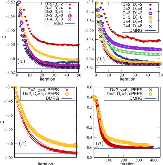
We also analyze the behavior of imaginary-time-energy optimization in the canonical PEPS form in the context of the ground state of the ITF and Heisenberg models. We also compare the results of direct energy optimization in the canonical form with results of standard PEPS optimization algorithms.
PEPS definition and background
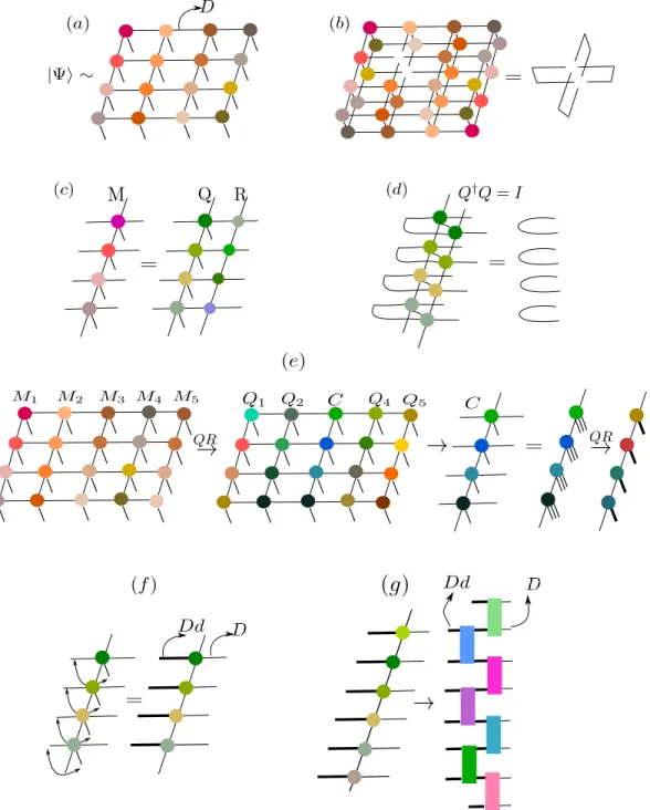
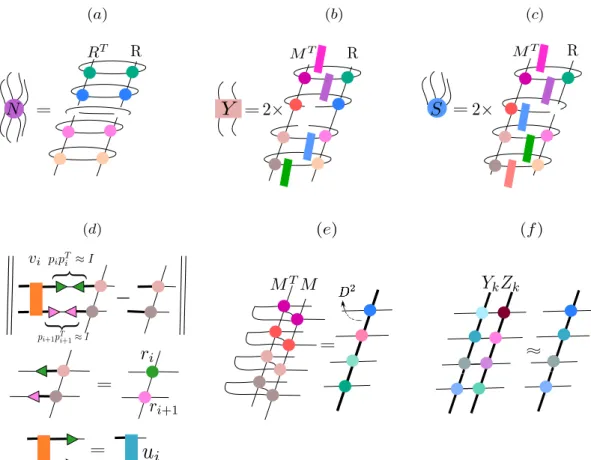
PEPS canonical form and column QR ansatz
The vertical bond dimension of the final 𝑌𝑘(𝑅) is compressed back to the original bond dimension 𝑀. The second is an absorption defect caused by shortening the vertical bond dimension of the central column to 𝐷𝑐.
Summary
This is because the mesh discretization of the correlation functions prevents radial isotropy in the basis {𝑓𝛽. The growth factor for the electric dipole moment of the electron in BaOH and YbOH molecules. Phys.
Efficient representation of long-range interactions in tensor net-
Abstract
We describe a practical and efficient approach to represent physically realistic long-range interactions in two-dimensional tensor network algorithms via projected entangled pair operators (PEPOs). This representation allows efficient numerical simulations with long-range interactions using projected entangled pair states.
Introduction
In 1D, the increased computational cost of long-range interactions can be eliminated if they are smooth and decaying. Based on these ideas, in this work we describe how general long-range interactions in two dimensions, including the Coulomb interaction, can be efficiently encoded as a sum of PEPOs evaluated by a low-rank correlation function.
Correlation function valued PEPOs
As a concrete example, consider the spin-spin correlation function⟨𝜎𝑖𝜎𝑗⟩ of the 2D Ising model, which has the Hamiltonian 𝐻 =−Í. 3.1(a)) is the operator-valued tensor in the Ising CF-PEPO and (𝐿𝑘, 𝑙𝑘) is a composite index of the relation 𝐿𝑘 for the 2D FSM and the relation 𝑙𝑘 of the Ising PEPS.
CF-PEPOs and the auxiliary lattice
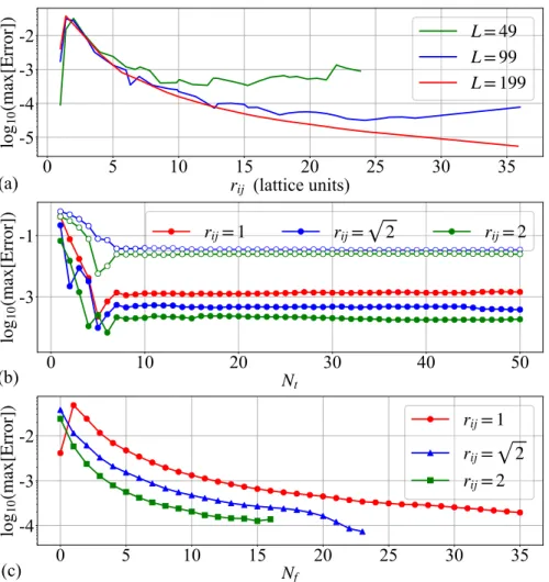
In summary, the full CF-PEPO is obtained by concatenating the FSM of the operators (either in serpentine form, or the full 2D FSM) with the Ising CF-PEPS on an extended mesh as specified by Eq. The total fitting error is controlled by the expansion parameter 𝑁𝑓 and the number of terms 𝑁𝑡.
Computational cost
The fits were performed on a disk with a radius equal to the maximum 𝑟𝑖 𝑗 shown for a given curve. Each ˆ𝑂𝑖 can be represented as a snake-like MPO with bond dimension𝐷 =3, and the cost of contracting a single ˆ𝑂𝑖 expectation value is then 𝑂(𝐴 𝜒3𝐷3 . 𝑆) with 𝜒∼ 𝐷 𝐷2.
Results
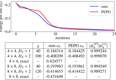
The fifth column is the overlap of the normalized ground states obtained with the two different methods. We observe that the trajectories are similar and the use of PEPO does not change the stability of the gradient optimization, although it requires a larger value of 𝜒.
Summary
In this section, we will focus on the nature of the nematic phase and its stability in the thermodynamic limit (TDL). This section describes the effect of the approximations made in the numerical in Ref.
A simplified and improved approach to tensor network operators
Abstract
To lower these two barriers, we describe how to reformulate a PEPO into a set of tensor network operators similar to MPOs, by taking into account the different sets of local operators generated from successive bipartitions of the 2D system. The expectation value of a PEPO can then be evaluated on-the-fly using only the action of MPOs and generalized MPOs at each step of the estimated contraction of the 2D tensor network.
Introduction
In this article, we describe how to overcome both the computational and conceptual complexity of using general operator representations of the tensor lattice Hamiltonian in 2D algorithms. In Section 4.5, we demonstrate this simplicity by reporting explicit gMPO forms for various representative types of 2D Hamiltonians.
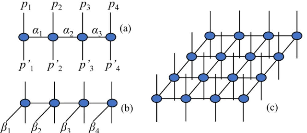
Matrix Product Operators (MPOs)
To understand these patterns, as well as the form of the MPO matrices in this section, we recommend Ref. These linear transformations can be found by taking SVDs of certain blocks of the upper triangle of 𝑉𝑖 𝑗.
PEPO expectation value via generalized MPOs
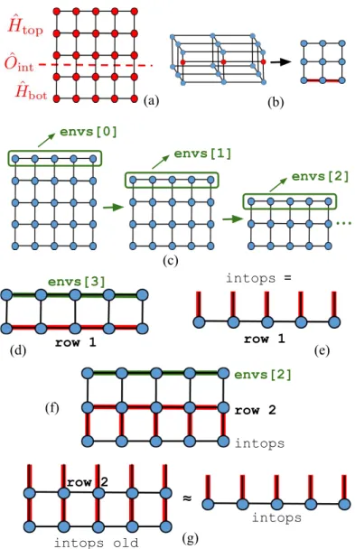
Then, these complementary operator matrices are applied between each of the bh and ket tensors in the row 𝑦 along the vertical indices. At each iteration of the algorithm, we first compute ⟨𝜓|𝐻ˆ|𝜓⟩ for the set of terms in the difference (1) - (3) by contracting a gMPO within tops, and then we construct a new intop for the next iteration that accounts for all the terms in (2) by slightly changing the preceding intopes.
Results
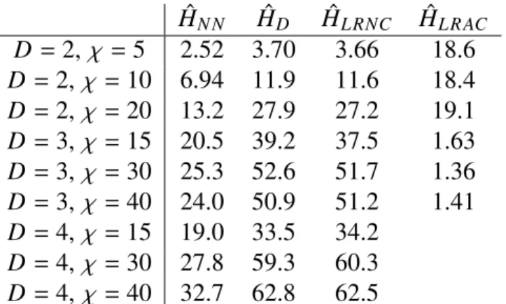
Consider a Hamiltonian with local 1-body terms and nonsymmetric nearest-neighbor interactions of the form, . For the operator ˆ𝐼 in the bottom row of the matrix, which combines the action ˆ𝐴(from the bottom) with the action ˆ𝐵(right) in the gMPO row, it is.
Summary
A factor of ~ 2 speedup can be achieved in step 4 of the gMPO boundary algorithm if we instead use non-symmetric gMPO tensors of horizontal dimension 𝐷 such that the interactions ˆ𝐴𝑥 , 𝑦𝐵ˆ𝑥 , 𝑦+𝑏+𝐴ˆ𝑥 , 𝑦+ 𝐴ˆ𝑥 , 𝑦𝐵ˆ𝑥 . 𝑎, 𝑦+𝑏 are encoded in one gMPO, and the interactions ˆ𝐴𝑥 , 𝑦𝐵ˆ𝑥−𝑎, 𝑦+𝑏 in another. The cost of this reduction in bond dimension is an increase in the number of gMPOs that must be independently evaluated from 𝐾 to 2𝐾, but this still leaves a factor of 2 for speedup because the cost of step 4 is quadratically dependent on the horizontal dimension of the gMPO bond.
Short Appendix
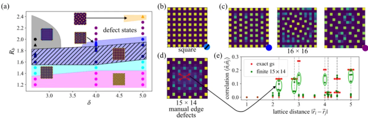
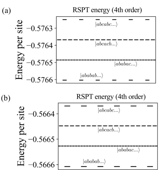
These are simply a consequence of the finite resolution used to sample the phase space in the phase diagrams. It is clear that the structure of the wave function (Figure 3c) does not correspond to a single dressed |𝑎 𝑏 𝑎 𝑏 𝑎 𝑏.
Entanglement in the quantum phases of an unfrustrated Rydberg
Abstract
We report on the ground state phase diagram of interacting Rydberg atoms in the geometrically unfrustrated square lattice array. We find a strongly altered phase diagram from previous numerical and experimental studies, and in particular we uncover an emergent entangled quantum-nematic phase that arises in the absence of frustration.
Introduction
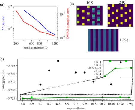
Furthermore, recent numerical results [134] highlight the sensitivity of the physics to the tails of the Rydberg interaction and finite size effects. By greatly varying the size of the DMRG supercell with the Γ point, it obtains many different ground states.
Numerical strategy and techniques
152], arbitrary isotropic interactions can be efficiently represented in this form, which mimics the desired potential via a sum of Gaussians, i.e. the combs can be efficiently contracted much cheaper than using a general tensor network operator. 152] described the Hamiltonian coding, we must also find the ground state here.
Bulk phases
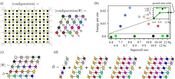
3 and 17 density gaps respectively, but the nematic phase also replaces the large region of the 16 density "3-star" crystal. The non-mean-field (entangled) character of the nematic phase is evident. c) Structure of the nematic state in terms of classical configurations constructed by compositions of 3 individual column states|𝑎⟩,|𝑏⟩,|𝑐⟩.
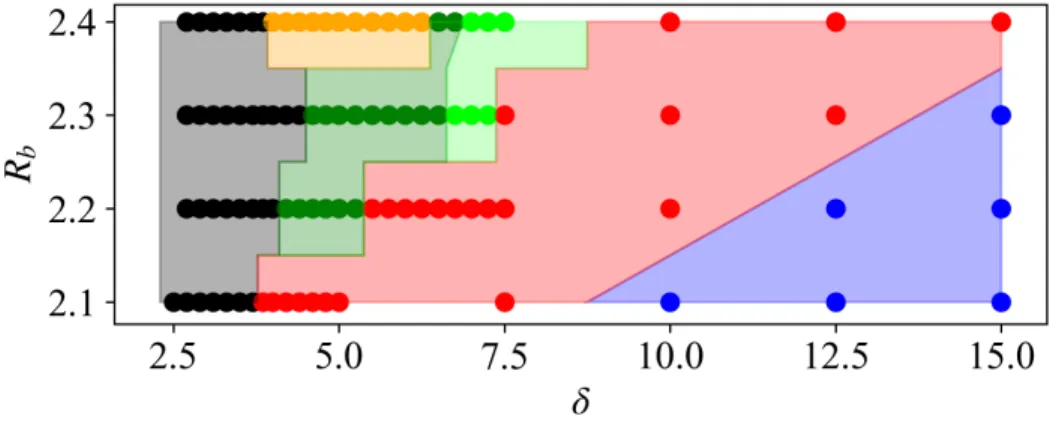
Finite phase diagram
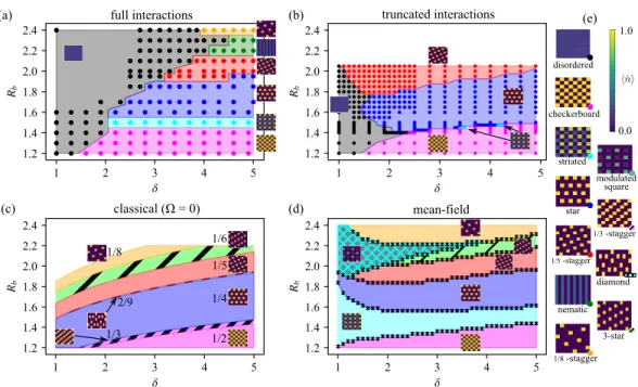
A new region of classical order, here called the square phase (Fig. 5.4b), emerges in much of the 𝑅𝑏=1.5−1.8 region where the stellar phase was mostly stable [145] . Our calculations support a reinterpretation of the experimental data with a significantly larger square/dashed area and a much smaller stellar phase.
Summary
Reducing the complexity of quantum chemistry methods by choosing a representation. Journal of chemical physics148,044106. U (1)-symmetric projected infinite entangled states- Study of the spin-1/2 square J 1- J 2 Heisenberg model.Pezical Review B97,174408.
Ultracold hypermetallic polar molecules for precision measure-
Abstract
Laser cooling is a powerful method to control molecules for applications in precision measurement as well as quantum information, many-body physics, and fundamental chemistry. To extend the control afforded by laser cooling to a wider set of promising atoms, we consider the use of small hypermetallic molecules containing multiple metal centers.
Introduction
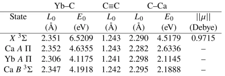
We discover that these molecules are linear and possess metal-centered valence electrons, and study the complex hybridization and spin structures relevant to photon cycling and laser cooling. Diatomic species such as BaF [176], RaF [182], TlF [173] and YbF [174] are thus promising candidates for laser cooling and are sensitive to new physics beyond the standard model.
Electronic Structure
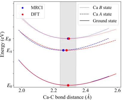
The structure of the lowest lying excited states consists primarily of 4𝑠𝜎 → 4𝑝 𝜋 transitions on the Ca atom (which we will call the Ca 𝐴 state), 6𝑠𝜎 → 6𝑝 𝜋 on the Yb𝐴 state, (which we will call it Yb𝐴) , and 4𝑠𝜎 → 3𝑑𝜎 on the Ca atom (which we will call the Ca 𝐵 state), which are the potential laser cooling transitions. These orbitals are constructed as the eigenvectors of the difference between the density matrices for .
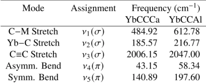
Vibrational Structure
Additionally, the effects of the "worst case" systematic error estimates for this transition are smaller: 0-0 FCF is reduced to 0.993, 4 total states are needed for an efficiency of 0.9991, and 7 total states are needed for an efficiency of 0.9999 . This limits the scattering efficiency of the Yb atom to ~500 photons with a reasonable number of repumping lasers, without even considering systematic errors or the additional lasers needed due to crossover between systems.
Computational Details
Shift in the y-coordinate is necessary because DFT and MRCI do not predict the same excitation energies. The ground state curves are virtually identical in the window of significance (marked in gray).
Discussion
Furthermore, the FCFs are calculated assuming that the potential energy surfaces in the immediate vicinity of the equilibrium geometries for the ground and excited states can be approximated by a harmonic potential. 233], so no assumptions were made that the normal modes of the ground and excited states are parallel.
Summary
First, the cycling center can be used for improved condition tracking to deliver improved statistics. Second, the cycling center provides an additional co-magnetometer that can be used to diagnose stray fields and other systematic effects.
Short Appendix
Generalization of the exponential basis for tensor network representations of long-range interactions in two and three dimensions.Phys. Zhuang, X. et al. Franck–Condon factors and radiative lifetime of the𝐴2Π1/2− 𝑋2Σ+ transition of ytterbium monofluoride, YbF.Phys.
Numerical methods
Another way to understand the 2D DMRG calculation in the Bloch basis is to examine the shape of the correlation functions it predicts for an infinite system. There are two types of finite size errors in the energy of the Γ-point formulation of the bulk Rydberg system.
Entangled nematic phase
This order of RSPT captures the ordered phase energies in the mean field with high accuracy. This reveals the origin of the classical exponential degeneracy that was previously discussed in the 2D system.
Bulk phase diagram degenerate region
These eigenvalues correspond to all possible arrangements of individual column states that do not violate any restrictions in Eq. In terms of the interpolation spectrum, we can apply the operator P to a simple product state | 𝜓0⟩(a𝐷 =1 MPS) containing an equal mixture of all possible column states i.e.
Bulk phase transitions
The small lime green region indicates the degenerate zone where the distance between the 3-star and nematic phase becomes very small.
Finite phase diagram: 15 × 15 and 16 × 16
(a) row directly reproduces the experimental phase diagram on the 13×13 lattice (data extracted from ref. The first three columns show all three order parameters used in [143] to distinguish the phase diagram, while the fourth column shows a new , more exact order parameter for the star phase.
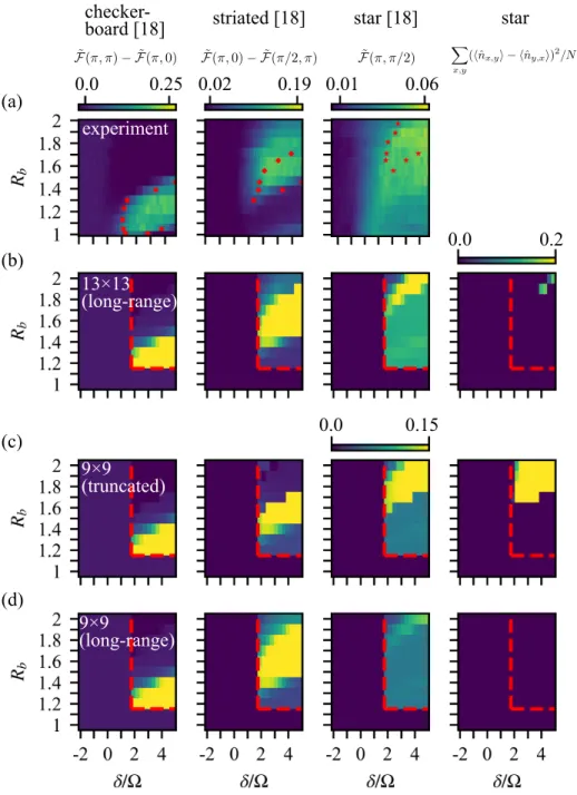
Comparing to experiment: 9 × 9 and 13 × 13 lattices
- Detailed tensor network diagrams corresponding to the steps of the
- Accuracy of the variational ansatz for QR decomposition of a single
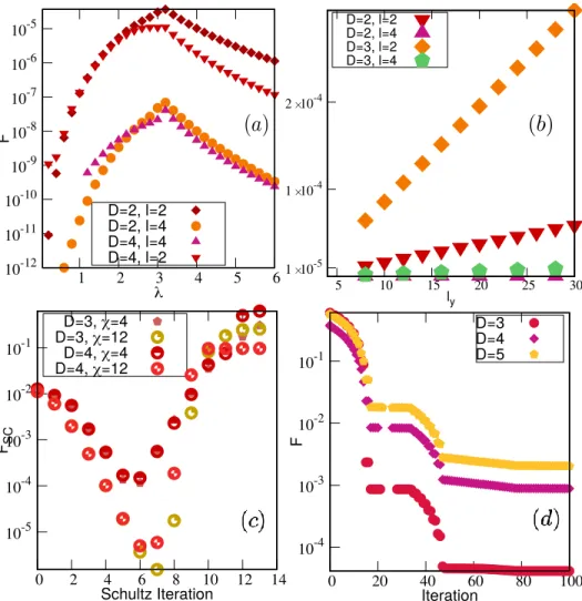
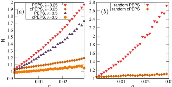
- Convergence of errors in the global norm of the PEPS
- Enhanced numerical stability of the canonical PEPS compared to a
- Ground state optimization for various models using the PEPS canon-
- Tensor networks diagrams detailing the layout of a CF-PEPO and the
- Convergence of the fitting procedure for the Coulomb potential using
- Accuracy of energy expectation values using the CF-PEPO
- Ground state optimization of a long-range Heisenberg model using
- Tensor network diagram of a generalized-MPO, compared to a typical
- Tensor network diagrams specifying the operator-valued elements of
- Simple example of how a gMPO contraction encodes a Hamiltonian
- The first full iteration of the boundary gMPO energy contraction
🝑 On a finite lattice, this provides a clean way to determine the phase of the star separately from the other orders in this group.
![Figure 3.1: (a) The construction of the nonzero parts of the CF-PEPO tensor W [𝑘] via the coupling of the finite state machine (FSM) tensor (red) with the Ising correlation function tensors (blue)](https://thumb-ap.123doks.com/thumbv2/123dok/10410800.0/49.918.185.726.98.554/figure-construction-nonzero-coupling-machine-correlation-function-tensors.webp)
![Figure 4.2: A set of tensor network diagrams that represent the elements of the operator-valued MPO matrix ˆ 𝑊 𝑔 𝑒𝑛 [ 𝑖 ] (a), along with the additional elements needed for ˆ 𝑊 𝑔 𝑒𝑛−𝑠 𝑦 𝑚 [ 𝑖 ] (b)](https://thumb-ap.123doks.com/thumbv2/123dok/10410800.0/65.918.208.711.97.486/diagrams-represent-elements-operator-𝑒𝑛-additional-elements-𝑒𝑛.webp)
