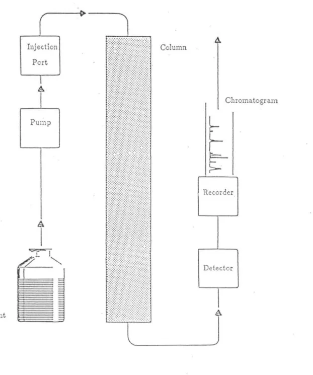
mathematical control theory for liquid chromatography

Another classical problem, solvent demixing, is explained in terms of a nonlinear multicomponent solvent model where the solvent gradient steepens with respect to adsorption and shock formation. At a specified time, a (perhaps unknown) mixture of chemicals dissolved in a chosen solvent is introduced to the "top" (higher pressure end) of the column and these solutions then flow down the column. Typically, at the bottom of the column, some sort of detector (eg, using light absorbance at a single wavelength or across a range of wavelengths) registers the solute concentrations during elution.

Hopefully, the chromatographic system is chosen so that all the solutes are dissolved when they arrive at the bottom of the column; if not, the system should be modified in some way. The surface of the particle is usually porous (see Figure 4) and the dissolved molecules diffuse into the pores and possibly adsorb to the solid surface of the substrate. The solvent can then displace the adsorbed molecule, which in turn can eventually diffuse out of the stationary phase back into the mobile phase.

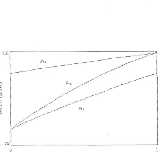
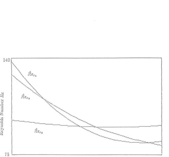
Due to the nature of the non-linear solvent equation, the solvent gradient will steepen if the gradient increases with time and flatten if the gradient decreases with time. See that the packing number appears in each of the dimensionless numbers, thus limiting the validity of the perturbation analysis to values.

Figure 1: Genera l T ypes of Chromatography.

CHAPTER 1

In order to find the dynamics of the solvent system, we must first consider the dynamics of the pressure gradient. The equation for the Hubbert potential for solvent gradient conditions in the case where the pressures are fixed at both ends of the column can be calculated as follows. We can now substitute this linear velocity form into the solvent dynamic equation.

The evolution of the norm is given as. using integration by parts if necessary). We have seen that the solution to the solvent equation is unique and exists; it can also be shown (28, and references therein) that there exists a unique solution to a linear partial differential equation of type . Substituting this into the integral of the Green function and integrating parts, we obtain.

Proof: (Although the argument can be carried through with D, =f 0, here we take D, = 0 for the clarity of the argument.) The form of the solute above the equation. Existence of solution to the solved equation: This follows by showing that the solution of the iteration equation given by. The shape of the function h(c) affects the profile of a concentration pulse moving down the column.

Initially, when the sample is introduced into the column, there are no adsorbed molecules.

Figure 5: Flow through an inclined chromatograp h column filled with a homo- homo-genecu.:; porous l1''!edi um

CHAPTER 5

The use of mole fractions in the above calculations presents some difficulties, especially when combining the solvent reaction model into the soh-ent continuity equation. The difficulty is that unless the two solvents have essentially the same chemical composition, the total number of moles cannot remain constant because the volume in the column is constant. Thus, we cannot simply divide the dynamics equation of each solvent by the total number of moles of solvents to obtain the dynamics of the solvent's mole fractions.

A more natural form of the concentrations is the volume fraction; there is a constant volume available to the mobile phase and a constant. Vie can take the molar concentrations appearing in each solvent equation and multiply by its partial molar volume, assumed constant, and thus we obtain the volume fraction of solvent per em3 column volume. However, we find satisfactory accuracy with experimental data, assuming that the partial molar volumes are constant, at least in the examples considered to date.

The form of substance isotherms in terms of volume fractions can be essentially the same as those in terms of mole fractions, the only difference being the reaction coefficient ("Langmuir coefficient"). So if we go back to the definition of the Langmuir reaction coefficient in terms of activity and assume that the activity coefficients cancel out. From the definition of partial molar volumes and the presence of constant volumes in the stationary and mobile phase, we can write

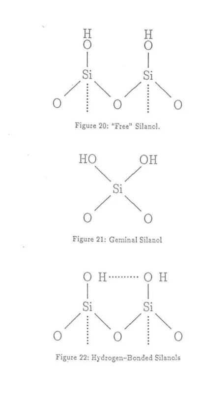
A two-dimensional schematic (Figure 23) of adsorbent silanols and the resulting polarity inhomogeneities shows what a polar solute can experience as it passes over the surface. The effects of inhomogeneities due to different types of silanols will be discussed in the next section in relation to solute and solvent equilibria. RPLC adsorbents consist of silica beads with one of the common functional groups attached to silanols.

Probably the most common functional groups are alkyl chains, often eight or eighteen carbons long. Silanols are never completely coercd, although the silanols are well below the alkyl "surface". Note that in contrast to the polar surface of NPLC, the bound surface of RPLC is apolar and hydrophobic. Thus, polar solutes will bind less than non-polar solutes, contrary to the characteristics of the NPLC adsorbent surface.

INCREAS ING POLARITY

Fine tune final procedure

Note that since D" v, and Pep vary with s, so do all of the above dimensionless quantities except c. This is done in the same way as in the solution for rn~; we simply choose the values of the initial conditions appropriately last term in the expression for dJ1.,jd( contains the factor dde which will be negative for the typical solvent gradient, thus reducing the peak width growth.

We want this time to be equal to the time when the end of the solvent gradient leaves the column. For the development of this research, it is important that the authors note that systems of n components with Langmuir isotherms can be represented as an (n + I)-component stoichiometric system. That a Langmuir system of the type considered by the authors is not inherently stoichiometric is easy to demonstrate; consider the following development of this.

In the next section, the applicability of the authors' formalism to our MPLC control problem will be discussed. The latter situation indicates the importance of being aware of the linear capacity of the column. 30J, is postulated to be of the form of the solution of a set of equations for chromatography.

Arnold made suggestions about the proper form of the flow rate dependence and for what values of u. If we accept the above phenomenological relationship, we can say that the plate number N, of the column must satisfy. The bandwidth near the end of the column can be expressed in length units relative to column length, so we give the expression.

Diffusion in the mobile phase results from the solute concentration gradient, and gives rise to a variance of where"{ is the tortuosity coefficient due to the structure of the substrate. What the equation does not include is the effect of interactions of the two types of localization. In fact, it is very likely the case that a large amount of controllability of the system is lost through medium.

This means that solutes near the top of the column experience a solvent gradient that is not as steep as the solutes. Exactly how important this nonlinear effect IS to the control of solute separation needs to be investigated.