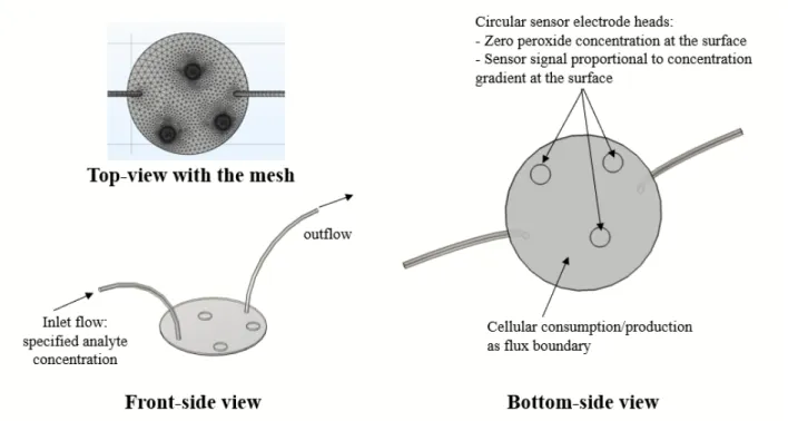
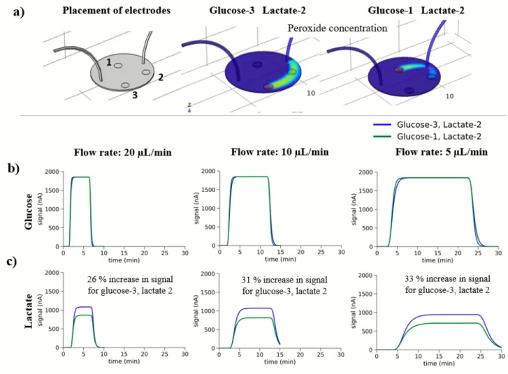
Fluid dynamics fine meshing was used for the geometry, including the size of the mesh elements in µm on the sensor surface (top view); convective flow boundary conditions determined at the inlet and outlet of the device (front view); the boundary condition was set to zero peroxide concentration on the sensor surface, assuming the electrode was fully consumed, and the cell consumption or production was set as the flux across the lower µCA surface. In an arrangement where the two electrodes are placed on the same side of the flow, the glucose signal interferes and increases the lactate signal by more than 20%, even higher with lower flow rates.
Overview and Specific Aims
To meet the research needs, a computational approach has been taken to develop predictive models for 1) the toxicokinetics in the device of PDMS-based organ-on-chip microsystems and 2) the cellular metabolite detection using the downstream microclinical analyzer. Detailed analysis of downstream detection will provide insight into the application of the microclinical analyzer to assess metabolic functions in organ-on-chip devices in response to toxic exposure.
Background and Significance
- Organ-on-chip microsystems
- Chemical-PDMS interaction in organ-on-chip microsystems
- Computational modeling for organ-on-chip microsystems
- Chemical detection techniques for cellular metabolism
- Electrochemical measurement of metabolites
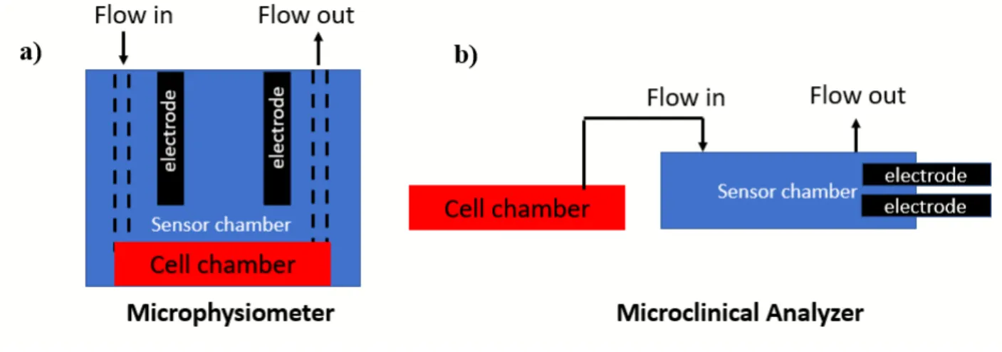
- Microphysiometer vs microclinical analyzer
Depending on the concentrations and speed of the reaction, part of the glucose is also converted into lactate. Follow-up detection refers to the real-time chemical analysis of OCM by directly linking the OCM to the detection method.
Organization of the Dissertation
Finally, Chapter 5 summarizes the main conclusions of the study and also provides recommendations for further study. Attempts are made to draw conclusions from the various findings of the study and the recommendations provide a basis for further studies.
Abstract
Auner, A.W.*, Tasneem, K.M.*, Markov, D.A., McCawley, L.J., and Hutson, M.S., "Kinetics of Chemical-PDMS Bonding and Implications for Bioavailability in Microfluidic Devices," Lab on a Chip, 2019, first author , *equal . These fitted parameters were used to model the impact of PDMS bonding on chemical transport and bioavailability under realistic flow conditions and device geometry.
Introduction
Here we provide a simple method for measuring the necessary model parameters for reversible and irreversible PDMS binding kinetics. Once the binding parameters are measured, we then present a model that combines computational fluid dynamics (CFD) with PDMS binding kinetics to predict chemical bioavailability in a simple microfluidic device.
Experimental design
- PDMS preparation
- Chemical preparation
- Assessing PDMS binding via UV-vis measurements
- Assessing PDMS binding via FTIR measurements
- Computational model
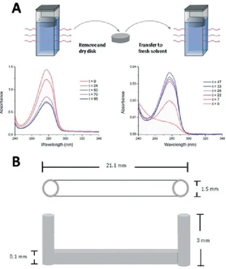
-right) UV-vis spectra showing the return of ethofumesate to bulk solution when desorbed into fresh solvent from a pre-soaked PDMS disk. UV-vis absorbance spectra for on and off experiments were measured against matched cuvettes with the appropriate solvent using a Cary 5000 dual-beam UV-vis spectrometer (Agilent, Santa Clara, CA; scan rate = 24 nm min−1; resolution = 1 nm).
Results
Predicted impact of chemical-PDMS binding
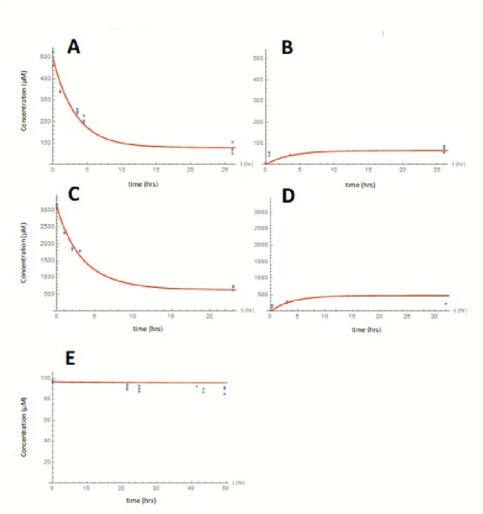
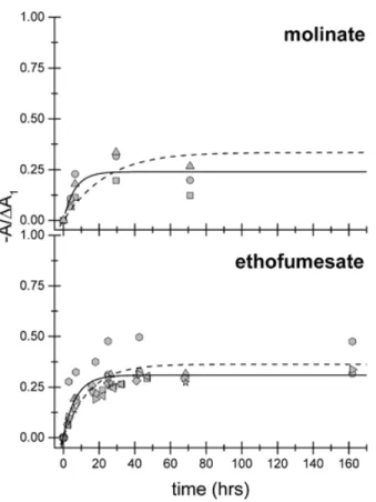
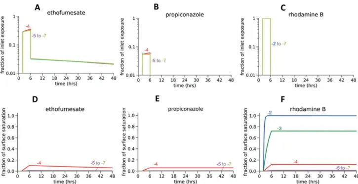
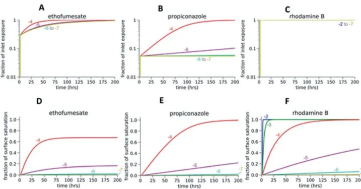
The microscopic model fits are shown alongside the empirical fits to the binding/desorption kinetics in Figure 2.2 and Figure 2.3. For a reversible binder such as etofumesate, the predicted cell exposure increases gradually with time and approaches the entry concentration asymptotically (Figure 2.5A). On the other hand, for an irreversible binder such as propiconazole, predicted cellular exposures approach nominal inlet concentrations only when the surface becomes fully saturated (Figures 2.5B and E).
Discussion
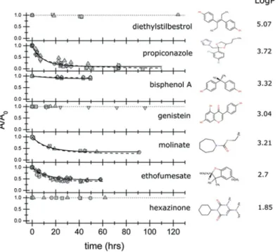
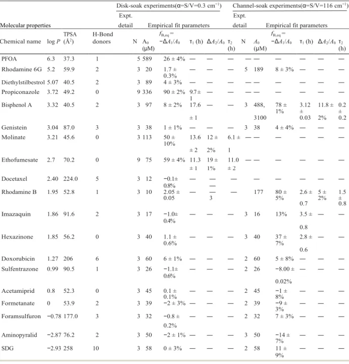
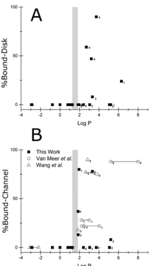
Despite agreement on the thresholds, we find that PDMS binding rate for chemicals with logP above (or TPSA below) the threshold is no longer linearly related to TPSA. Among these and 15 other molecular properties cataloged by ChemSpider (http://www.chemspider.com), the best predictor of PDMS binding was logP above the specified threshold and the number of H-bond donors (T-test P-value = 0 .0037). First, for three of the five PDMS-binding chemicals tested here, the PDMS carrier capacity exceeded 1000 molecules per nm2.
Conclusions
Modeling In-Device Toxicokinetics
Implementing Diffusion into Bulk PDMS in the Toxicokinetic Model
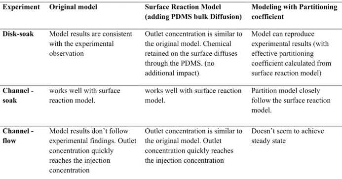
The original model was then compared with a surface reaction model and a partitioning model by simulating disk and channel wetting experiments. Surface reaction model, compared to the original model, the final concentrations were found to be the same. This is due to the similar approach of these two models to the use of binding kinetics on the PDMS surface, with the exception of the surface reaction model with additional diffusion into the bulk.
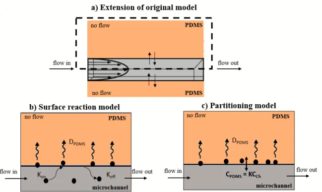
Geometry Development in Extended Models
Preliminary Analysis of Extended Modeling Approaches
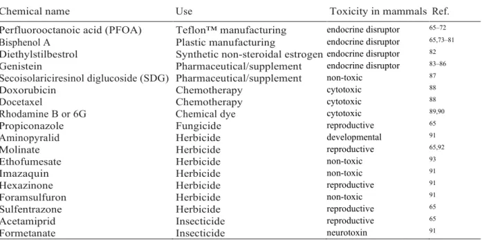
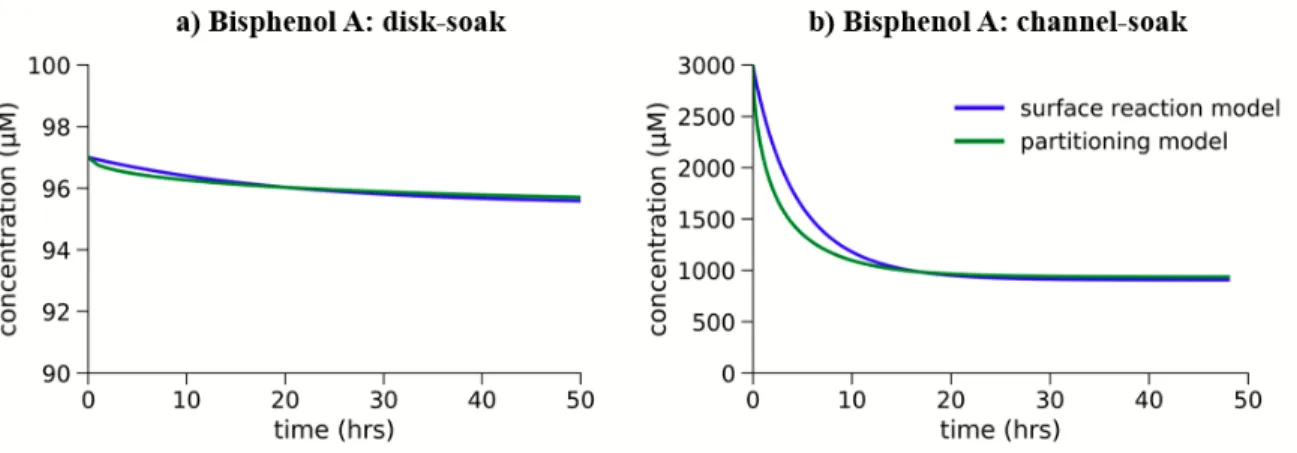
Bisphenol A
Similarly, the surface response model was run to simulate the channel absorption experiment, with an initial concentration of 3000 μM. In contrast to the disk wetting result, the predicted concentration depletion was large on the channel wetting length scale—as expected due to the larger surface-area-to-volume ratio. With an initial concentration of 3000 μM in the surface reaction model, higher depletion with higher α was predicted (Figure 3.5).
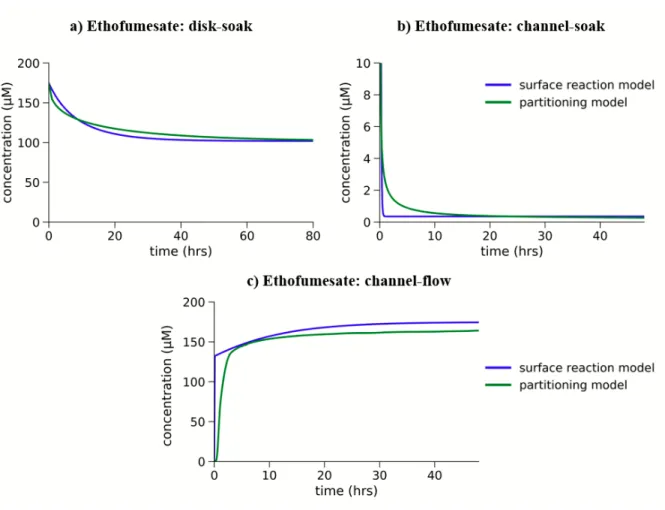
Ethofumesate
In addition to disk and channel soaking simulation, a model was developed for ethofumesate depletion in the channel flow experiment, especially for predicting the concentration at the channel outlet as done in the actual microfluidic experiments. Due to the continuous exposure of etofumesate, both surface response and partitioning model predicted the concentration to reach the nominal concentration (Figure 3.6). The findings under flow condition cannot therefore be conclusive without further analysis and validation with channel flow experiments.
Preliminary Experimental Design for Model Validation
Overall, in the long-term binding experiment, a steady release of the chemical from solution was evident, which is also inconsistent with the predicted concentration in Auner et al. (2019) and the model presented here in Figure 3.6c. This means that the interaction between chemicals and PDMS is far from saturation due to the rate-limiting kinetics of chemical binding-dissolving with PDMS. The chemicals were found to interact with the tygon tubing system, which was later replaced with the more chemically resistant perfluoroalkoxy (PFA).
Discussion
The orders of magnitude larger relative surface area means that the distribution of a chemical in the PDMS surfaces of microfluidic channels can drastically change a chemical's concentration in the perfusion solution34,43. As also discussed in Chapter 2, the previous modeling approach provided no way to separate the contributions of surface distribution of a chemical in PDMS and its distribution in the PDMS bulk. The binding capacities for some of the chemicals in the previous work were too large to represent a true surface carrying capacity thus implying a significant diffusion into the PDMS bulk.
Conclusion
Introduction
Enzyme-based Sensors for Metabolite Detection
To determine the peroxide consumption, the flux can be calculated using Equation 4.4 where I is the current generated by peroxide, n is the number of electrons transferred in the reaction (n =2 for redox-sparing metabolites and respective enzymes ), F is the Faraday's constant. W is the working area (in this case, circular head of the electrodes), and J is the molar rate of transfer. Here brackets indicate concentrations, A is the chemical substance/analyte (glucose/lactate/ . glutamate), P is the peroxide (H2O2), E is the enzyme, kF, kR and kcat are the reaction rate constants, Vmax is the maximum rate of the reaction and Km is the Michaelis Menten constant equal to the analyte concentration at which the reaction rate is half of Vmax.
Microclinical Analyzer Modeling using COMSOL
Geometry for the metabolite detection
The measured current signal resulting from the change in glucose, lactate or glutamate concentration at the enzyme-modified electrodes generates analytical data as current versus time. These data can be translated in terms of analyte concentration and exposure time, providing real-time information on metabolic activities.
Modeling enzymatic reaction in µCA
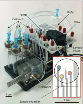
57. Figure 4.1 a) COMSOL geometry of two µCAs (radius = 6 mm, height of each chamber = 0.23 mm) connected with 150 mm tubes – the upstream chamber mimicked the cell chamber and the downstream chamber mimicked the µCA ; b) The circular section in the chamber shows a circular area of three electrodes (area = 1.8 mm2).
Boundary conditions
The transport of chemical species i from the cell chamber to the sensor chamber can be defined as convective-transport-reaction equation: 𝜕𝜕𝜕𝜕𝜕𝜕𝑑𝑑 = 𝐷𝐷𝑐𝑐∆2𝐢𝐢𝐢𝐶 𝐶𝐶𝑐𝑐 +𝑅𝑅, which is very similar to Eqs. The consumption of glucose and glutamate was defined as the molar flux (mol/m2.sec) at the electrode surface and those terms were normalized with the initial concentration. Lactate production terms were defined as a function of glucose production rate, including a measure of anaerobity (x%) of the cellular.
Estimation of Kinetic Parameters for Enzymatic Reaction
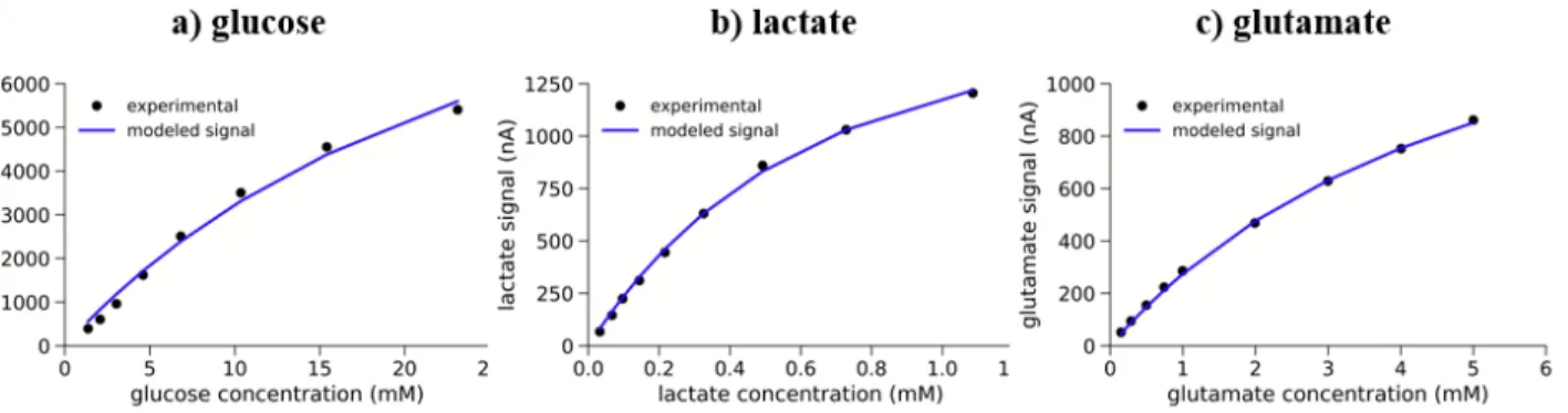
The objective function was defined as the goodness of fit (sum of squared residual) of the modeled calibration plots with the experimental data points (see Figure 4.4). For a given chemical, data from the calibration experiments were fitted to equation 4.6 and goodness-of-fit was assessed to compare with the quality of the literature results and this numerical approach. The details of the numerical method and the iteration results are included in the supplementary figure (S.6) and tables (S.7, S.8, S.9).
Downstream Metabolite Detection for Continuously Perfused System
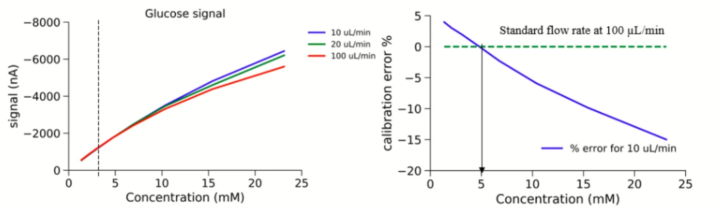
Predicted impact of flowrates in continuous perfusion
For high concentration, measurement at low flow rate is subject to calibration error up to 15%. Higher flow rates cause higher input of chemicals and low flow rates provide longer residence time for the reaction to occur. At high concentration, lower flow rate causes higher residence time for more peroxide production, increasing the signal.
Modeling Crosstalk in Metabolite Sensing
At a low concentration, higher flow rates produce a higher signal due to the faster availability of the glucose. If the flow rate of 100 µL/min is considered standard, calibration at 10 µL/min at a higher concentration would cause an error of up to 15% (Figure 4.5). There is no detectable change in glucose signals in the sensor setup.
Modeling Downstream Glutamate Consumption
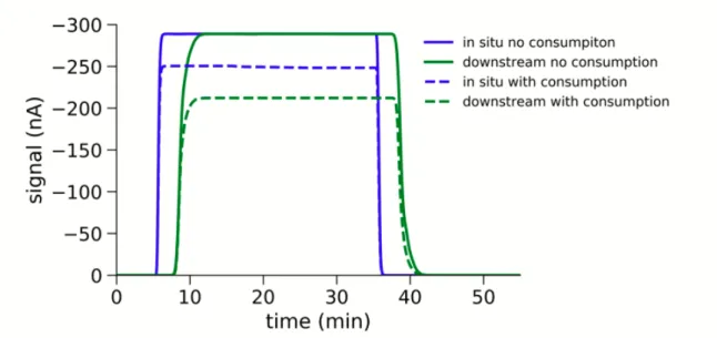
The model showed that the in situ cellular uptake of glutamate is 177.5 nmol compared to the downstream measurement of 177 nmol. Due to the cellular uptake of glutamate, the in situ signal was found to be 248 nA and the downstream signal was 212 nA. So, considering the flow condition and the exposure time, it was possible to simulate the experimental consumption in situ and to detect the glutamate consumption downstream of the cellular chamber without any discrepancy.
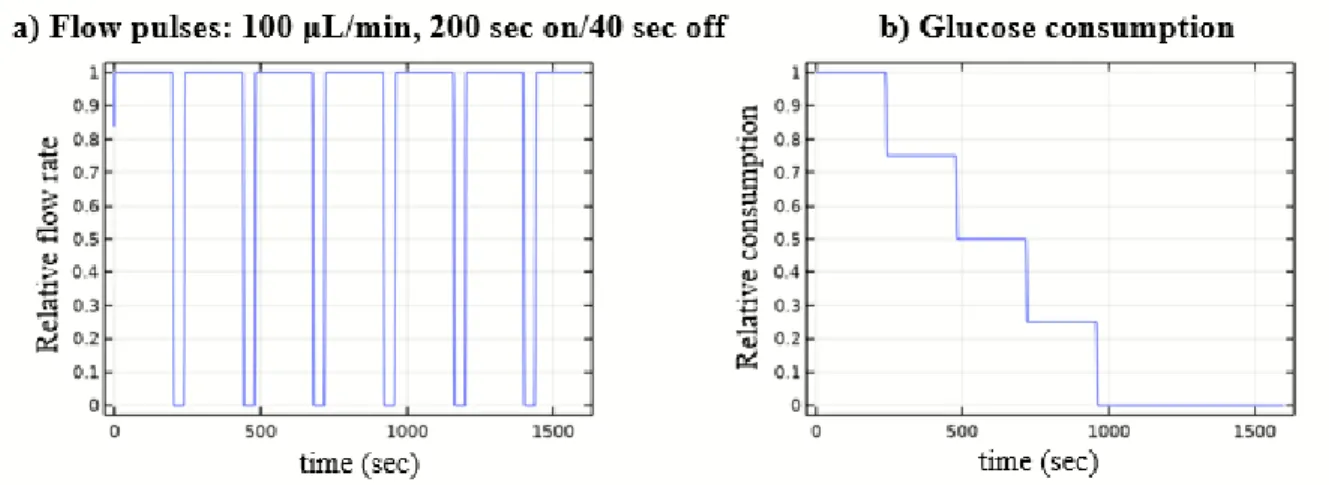
Modeling Metabolite Signals in Stop-flow Perfusion
The glucose signal dropped in the flow phase (starting from the 2nd cycle) due to the consumption on the upstream cell chamber in the previous stop phase. Here, the lactate production and glucose consumption during the stop phase can be determined by the peak height in the flow phase. With half the original volume of the first microchamber, both glucose and lactate signals increased approximately 40%, as seen in Figure 4.13.
Discussion
With lower volume of the cell chamber, the downstream signals are clearer and more characteristic.
Conclusion
Conclusions
If the model predicts any detection limitation for using sensors downstream of the cellular construct, this can be explored computationally to identify the alternative operating conditions for improved detection with higher spatiotemporal resolution. This computational effort will guide the researchers on design improvement for the next generation metabolite detection device for its application to organ-on-chip microsystems.
Future Directions
In-device toxicokinetics
This challenge certainly provides an opportunity for a future experimental approach to determine the diffusion coefficient for chemicals under liquid conditions. With the appropriate diffusion coefficient experimentally measured, the model can be run with kinetic parameters to obtain a range of areal density results that should be consistent with experimental measurements and model observations at different length scales. Other possible future work includes an experimental approach to evaluate the surface treatment of PDMS and study the damping behavior of the chemical-PDMS interaction for a wide range of chemicals of interest in toxicological study.
Metabolite detection
In utero exposure to bisphenol A alters the development and tissue organization of the mouse mammary gland. If the reflected point is still the worst of the three points, try two *contracted*. If the contracted sites are still the worst of the three points, *shrink* the simplex.