It would be easy for the instructor to select from these chapters a few topics of particular interest to supplement, if desired, the types of systems studied in the earlier part of the book. We hope that this book will continue to provide useful information for engineers involved in the analysis, simulation, and control of the devices of the future.
INTRODUCTION
- MODELS OF SYSTEMS
- SYSTEMS, SUBSYSTEMS, AND COMPONENTS
- STATE-DETERMINED SYSTEMS
- USES OF DYNAMIC MODELS
- LINEAR AND NONLINEAR SYSTEMS
- AUTOMATED SIMULATION
For example, events in the future do not affect the current state of the system. How many variables do you think are needed to fully describe the motion of the system.
MULTIPORT SYSTEMS AND BOND GRAPHS
- ENGINEERING MULTIPORTS
- PORTS, BONDS, AND POWER
- BOND GRAPHS
- INPUTS, OUTPUTS, AND SIGNALS
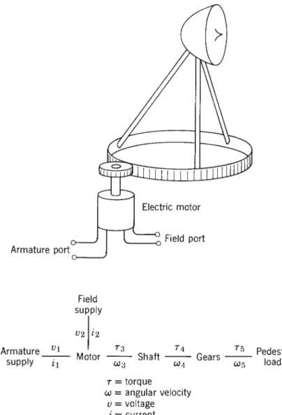
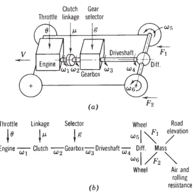
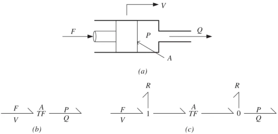
When using diagonal lines, judgment is required to place the effort and flow variables. For each of the multiple ports in Figure 2.1, construct a word-link graph similar to the one shown in Figure 2.3.
BASIC BOND GRAPH ELEMENTS
BASIC 1-PORT ELEMENTS
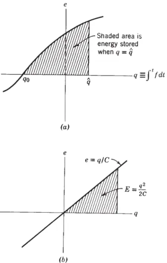
Because linear models are of great use in certain fields (for example, vibrations and electrical circuits), the linear versions of resistance relations in different energy domains are shown in Table 3.1, using the same notation as in Chapter 2. The units of the linear resistance parameter are simply the units of effort divided by units of power. For the linear case, it is usual to indicate the compliance parameter on the binding graph, as shown in Figure 3.2. a) Bond chart symbol; (b) defining the relationship;

BASIC 2-PORT ELEMENTS
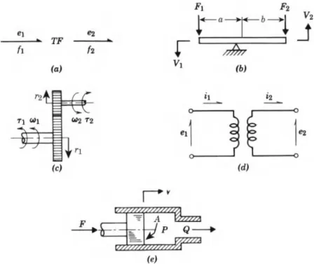
Similar limitations can be made on the validity of the transformer as a model for other physical devices. At any moment, energy is stored in both ports, but the characteristics of the device change.
THE 3-PORT JUNCTION ELEMENTS
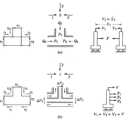
Using the inward force sign convention shown in the last version of the join implies that . 3.18). In words, the efforts on all bonds of a 0 junction are always identical, and the algebraic sum of the flows always vanishes. Depending on the orientation of the sign convention half-arrows on the bonds, minus signs or plus signs will appear in the equations of the junction.
The series and parallel aspects of junctions are more apparent in electrical cases than in mechanical ones. A 0 or 1 n-port junction has a common effort or drain across all links, and the algebraic sum of the complementary power variables in the link vanishes. In this case, both connections have the same flow, but one effort is the negative of the other.
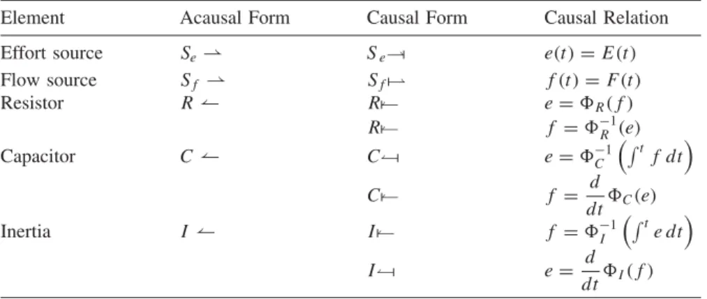
CAUSALITY CONSIDERATIONS FOR THE BASIC ELEMENTS The concept of causality was discussed in general terms in Section 2.4, and we
- Causality for Basic 1-Ports
- Causality for Basic 2-Ports
- Causality for Basic 3-Ports
Taking the capacitor, we can rewrite the relations of Table 3.2 as follows:. in which causality is implied by the form of the equation. Since inertia is the dual∗ of the capacitor, similar effects occur with the two choices of causality. The causal properties of 3-port 0 and 1 junctions are somewhat similar to those of the basic 2-ports.
Conversely, if all fluxes in all but one link are inputs to junction 0, the flux in the remaining link is determined and must be an output of the junction. Thus, if the flux at any single link is an input to junction 1, the fluxes at all other links are defined and must be considered outputs of the junction. Otherwise, when the efforts on all but one link are inputs to junction 1, the effort on the remaining link is determined and must be a product of the junction.
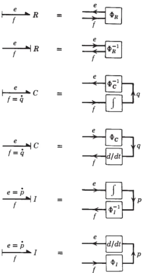
CAUSALITY AND BLOCK DIAGRAMS
When causal links are added to a connection graph, the information in the connection graph can be represented with a block diagram. It should be possible for you to relate the signal flow paths in the block diagrams to the equations in the tables and the connection diagram representation. Since the procedures for building linkage graph models and adding causal shocks to them are discussed in the following chapters, one option is to construct a block diagram from the linkage graph.
If P is the pressure at the bottom of the tank and Q is the volume flow, the tank is approximately —C for slow changes in the volume of the liquid stored. A rigid pipe filled with an incompressible fluid of mass density ρ has length and cross-sectional area A. If P1 and P2 are the pressures at the ends of the pipe and the volume flow rate is Q2, verify that the circuit diagram shown correctly represents a frictionless pipe. Prove that the constitutive law that relates the kinetic energy of pressure and volume flow is correct. by writing Newton's law for a fluid in a pipe.
SYSTEM MODELS
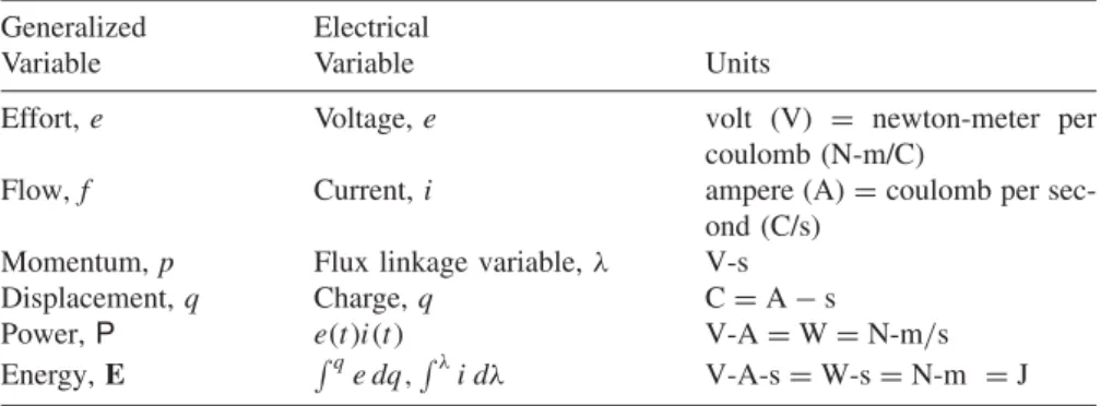
ELECTRICAL SYSTEMS
- Electrical Circuits
- Electrical Networks
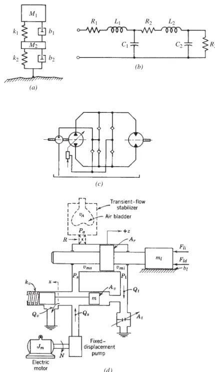
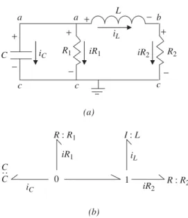
Label each node voltage on the circuit's schematic diagram and use a 0 junction to represent each node voltage, as shown in Figure 4.2b. Finally, the —I and —C elements associated with L1 and C2 are coupled to this 0 junction, yielding the binding graph of Figure 4.2e. Figure 4.3a shows the positive voltage drop and current directions, along with labels for the node voltages.
In Figure 4.4b, 1 connections are used to establish the positive voltage drop across the input and output sides of the transformer. This is deleted in Figure 4.5d, and connection graph simplifications were performed to produce the final result. The rest of the network is processed in Figure 4.6 in the same way as in the previous examples.
MECHANICAL SYSTEMS
- Mechanics of Translation
- Fixed-Axis Rotation
- Plane Motion
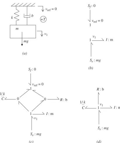
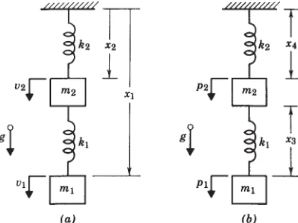
The power arrow is directed away from the 1-junction and into the source because if the respective mass element is moving upward (positive by assumption) and gravity is acting downward (as it always should), then the force flows from the system into the source, that represents gravity. The gravity source in the first example had a different sign convention because the absolute velocity there was defined to be positive downward, whereas the velocities here are positive upward.). The weight of the body is a source of stress associated with the vertical 1-cross with center of mass. The cylinder is a rigid body of mass, mc, with center of mass at the center and the moment of inertia about its center of mass, Jc, and has radius R.
4.6) with the velocity of the point at the end of the cylinder, vp, positive on the right, gives. In Figure 4.17, the velocity vector of the center of mass was split into two mutually perpendicular components aligned in the inertial XY directions. As an example of using body-fixed coordinates, consider the system in Figure 4.22a.
HYDRAULIC AND ACOUSTIC CIRCUITS
- Fluid Resistance
- Fluid Capacitance
- Fluid Inertia
- Fluid Circuit Construction
- An Acoustic Circuit Example
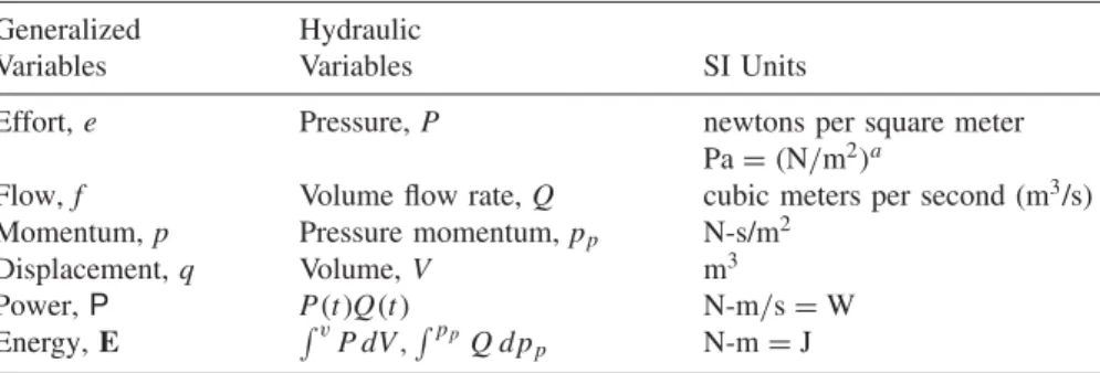
In this case a theoretical value for the resistance can be given, (see Reference [4], Section 7.4):. where μ[Pa·s] is the viscosity coefficient of the liquid, l [m] is the length and d [m]. As shown in Table 3.2, a liquid condenser imposes a relationship between a pressure (an effort variable) and the integral of the volume flow rate (a displacement variable). Most importantly, V3 according to Eq. 4.31), would represent the decrease in fluid volume in the pipe segment.
The minus sign in Eq. 4.37) is due to the fact that when the volume of the liquid increases stepwise by an amount of dV, the pressure decreases by the amount of dP. The incompressible liquid stream, Q3, compresses the gas in the bladder, and the volume of the compressed gas determines the pressure in the accumulator and at the 0 junction. A simple derivation of the coefficient of inertia for this case involves writing Newton's law for the fluid in the pipe.

TRANSDUCERS AND MULTI-ENERGY-DOMAIN MODELS
- Transformer Transducers
- Gyrator Transducers
- Multi-Energy-Domain Models
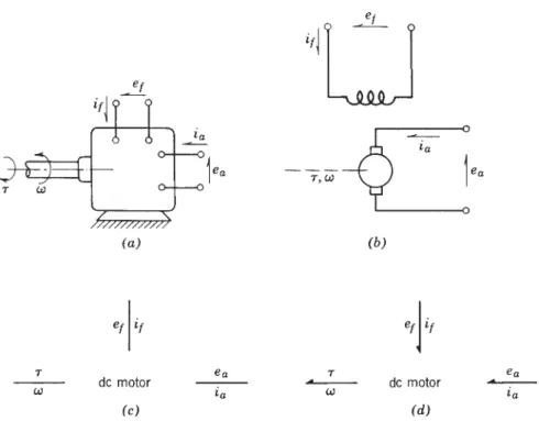
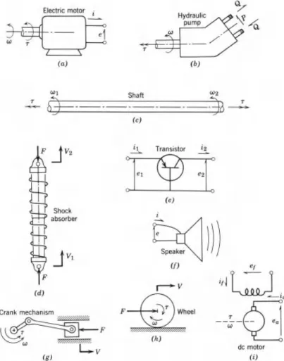
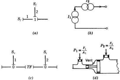
In fact, the ideal transformer transducer really only applies to piston face effects. The ideal pump or motor model is shown in the form of a connection diagram in Figure 4.32b. Furthermore, the torque produced is proportional to the current at the device terminals.
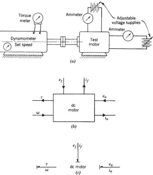
The left side of the v delubre connection graph represents the voltage source and the DC motor. Make a connection graph model of the network using the active 2-port as the coupling element. The ideal form of the device shown is a transformer as shown in the circuit diagram.
STATE-SPACE EQUATIONS
AND AUTOMATED SIMULATION
STANDARD FORM FOR SYSTEM EQUATIONS
One of the most remarkable features of connection graphs is that a study of equation formulation can be performed before any equation is written. Many important mathematical problems, methods, and results are organized according to the first form. An interesting example of the third form is found in the sets of second-order equations generated by the Lagrangian approach to system analysis.
In principle, a transformation from one of the given forms to any other is possible, regardless of whether the system is linear or non-linear. For linear systems, equations of the form (5.11) can be put into a standard matrix formulation. where X is a vector of state variables, . This simply means that given the values of the arguments on the right-hand side of Eq. 5.4), the set of values for the derivatives can be found by algebraic means.
AUGMENTING THE BOND GRAPH
For each of the 2-port junction elements, TF and GY, there are two possible causal forms that preserve the basic definition of the element. Bond graphs "keep track" of energy, and the instantaneous energy of the system is indicated by the energy variables (p's on -I's and q's on -C's) associated with the energy storage elements. Knowledge of the energy variables determines the energy state of the system at each instant of time.
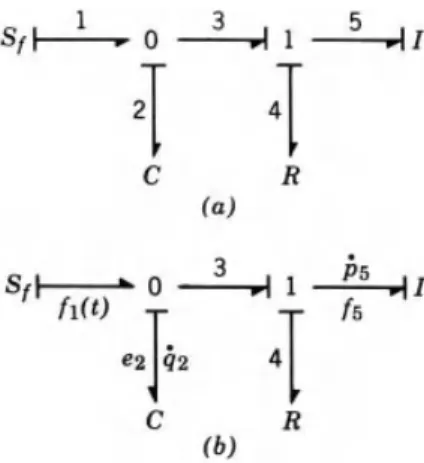
Further discussion of the use and interpretation of causality in more complex linkage graphs is given in Chapter 7. In part b of Figure 5.4, bond 1 is directed according to the meaning of the source element (a source of flow). Immediately, binding 3 must be causally directed because of the 0 junction, which can have only one effort input, e2.
BASIC FORMULATION AND REDUCTION
The notation f1(t) can be used to remind us that f1 is a well-known input function of time.) The current f3 is not wanted in the formulation, so we need to look further. The current, f5, is a co-energy variable and is directly related to the state variable p5, through the constitutive relation for the element. The effort, e2, is an output of the 1 split and is caused by e1, e3, ande4, by power convention; So,.
trye4 is an output from node 0 and is caused by the causal input,e5. Flowf4 is the output from node 1, caused by the co-energy variable, f2, where. The flux f10 is the output flux from the transformer, caused by the input flux, f11, according to. 5.42).
EXTENDED FORMULATION METHODS—ALGEBRAIC LOOPS Constructing models of physical systems always requires modeling assumptions
- Extended Formulation Methods—Derivative Causality
Let's see what happens if we try to derive the equations of state using the procedure in the previous section. It is a direct result of the modeling assumptions that went into the schematic in Figure 5.10a. When a resistive element is involved in the loop, it is customary to select the variable that was arbitrarily chosen to be the output of the R element and the input to the rest of the system.
When derivative causality arises, the state equations become implicit, meaning that some of the state variable derivatives. Thus, knowledge of the independent state variables allows algebraic determination of the energy variables on the derived elements, and thus calculation of their contribution to the system energy. It was decided, for this application, that the rotational inertia of the motor is negligible and it is not included.