Jurnal Nasional Pendidikan Teknik Informatika : JANAPATI | 304
MULTILEVEL THRESHOLDING OF COLOR IMAGE SEGMENTATION USING MEMORY-BASED GREY WOLF OPTIMIZER WITH OTSU
METHOD, KAPUR, AND M.MASI ENTROPY
I Made Satria Bimantara
1*, Anny Yuniarti
21,2Departemen Teknik Informatika, Institut Teknologi Sepuluh Nopember email: [email protected]1, [email protected]2
Abstract
Determining the optimal threshold value for image segmentation has become more attention in recent years because of its varied uses. Otsu-based thresholding methods, minimum cross entropy, and Kapur entropy are efficient for solving bi-level thresholding image segmentation problems (BL-ISP), but not with multi-level thresholding image segmentation problems (ML-ISP). The main problem is exponentially increasing computational complexity. This study uses the memory-based Gray Wolf Optimizer (mGWO) to determine the optimal threshold value for solving ML-ISP on RGB images. The mGWO method is a variant of the standard grey wolf optimizer (GWO) that utilizes the best track record of each individual grey wolf for the global exploration and local exploitation phases of the problem solution space. The solution candidates are represented by each grey wolf using the image intensity values and optimized according to mGWO characteristics. Three objective functions, namely the Otsu method, Kapur Entropy, and M.Masi Entropy are used to evaluate the solutions generated in the optimization process. The GridSearch method is used to determine the optimal parameter combination of each method based on 10 training images. Evaluation of the performance of the mGWO method was measured using several benchmark images and compared with five standard swarm intelligence (SI) methods as benchmarks. Analysis of the results was carried out qualitatively and quantitatively based on the average PSNR, RMSE, SSIM, UQI, fitness value, and CPU processing time from 30 tests. The results were analyzed further with the Wilcoxon signed-rank test. The experimental results show that the performance of the mGWO method outperforms the benchmark method in most experiments and metrics. The mGWO variant also proved to be superior to the standard GWO in resolving multi-level color image segmentation problems. The mGWO performance results are also compared with other state-of-the-art SI methods in solving ML-ISP on grayscale images and was able to outperform those methods in most experiments when combined with the Otsu method and Kapur Entropy.
Keywords : Multilevel Thresholding, Color Image Segmentation, Memory-based Grey Wolf Optimizer, Otsu Method, Kapur Entropy, M.Masi Entropy
Received: 06-06-2023 | Revised: 24-07-2023 | Accepted: 26-07-2023 DOI: https://doi.org/10.23887/janapati.v12i2.62874
INTRODUCTION
Image segmentation plays an important role in advanced image processing [1], [2] and computer vision [3], [4]. Image segmentation has been utilized in terms of satellite imaging [5], automatic target recognition [3], [6], [7], and medical image analysis [8]–[11]. Good image segmentation can determine the performance of advanced image analysis [6]. The thresholding method is the most commonly used approach to perform image segmentation [3]–[8], [12]–[18].
The thresholding method is commonly used for image segmentation because of its simplicity and efficiency [3], [6], [7], [15], [19].
The main objective of the thresholding method is to determine the optimal threshold value so that it can divide the image into several
regions based on the pixel intensity value of an image. Thresholding methods can be divided into two based on the number of values taken from the histogram of an image, namely bi-level thresholding and multilevel thresholding [3], [6], [18]. When the selected threshold value is one, it is known as bi-level thresholding, whereas when more than one threshold value is selected, it is known as multilevel thresholding [6].
The non-parametric approach to the thresholding method which uses certain criteria to obtain the optimum threshold value has been proven to be better for solving BL-ISP [6]. Otsu's between class variance, minimum cross entropy, Kapur entropy are some of the criteria commonly used to complete BL-ISP [3], [6], [13].
Although these criteria have proven to be very
Jurnal Nasional Pendidikan Teknik Informatika : JANAPATI | 305
efficient in solving BL-ISP on grayscale images, this approach has proven to be inefficient [20]
and impractical [3] to be used to solve ML-ISP.
Computational complexity will increase exponentially [7], [14], [15], [20] as the number of specified thresholds increases [3], [4], [6], [7], [14], [15] and performance levels tend to decrease [6]. This is because all possible threshold value pairs must be tried thoroughly in order to meet the specified criteria. Therefore, determining the optimal threshold value at ML- ISP in a short time is a challenge [7].
Determining the optimal threshold value for ML-ISP is included in the NP-hard combinatorial optimization problem [6], [7], [13], [18] and has been a challenge in the last few decades [7], [18]. Several approaches have been proposed to solve this problem, including using an SI-based metaheuristic optimization algorithm. The metaheuristic algorithm is proven to be more efficient in finding the optimal threshold value for solving ML-ISP when compared to exhaustive search [3], [6], [13], [15]. SI-based metaheuristic algorithms have been widely used to reduce computational complexity and have proven to be more accurate in solving ML-ISP when compared to evolutionary algorithms [3].
The Otsu, Kapur Entropy, and M.Masi Entropy methods have each been used as an objective function to solve ML-ISP on grayscale images with various proposed SI-based methods. Otsu's method with GA-PSO [20], MFO [18], KHO [15], WOA [18], GWO [14] and improved WOA [4] have been tried before.
Kapur Entropy with WOA-SMA [8], multistage hybrid SI optimization algorithm [6], DA [3], GWO [14] and KHO [15] have been tested before. M.Masi Entropy with GWO [7] and PSO [3] have been tested before.
Problems arise when there is no one optimization method that can provide the same solution for all optimization problems referring to the No Free Lunch (NFL) theory [7]. Several previous studies that utilized the SI method to solve ML-ISP [3], [4], [6]–[9], [15], [20], [21] only tested the method they proposed using one function. just be objective. In fact, it is important to test the robustness and consistency of the performance of the proposed method against different objective functions. Thus, it can be guaranteed that the performance of the proposed SI method is stable against several objective functions used [7].
In addition, many studies that apply the SI method to solve ML-ISP only focus on grayscale images as their test images [2], [3], [6]–[9], [14], [15], [17], [18], [20], [21]. In fact, color images can provide a better description of
an image than grayscale images [13]. Research related to the completion of ML-ISP using SI on color images is very little found [4], [13]. Ma dan Yue (2022) [4] have implemented a variant of WOA to solve ML-ISP on color images.
However, this study did not explain in detail the steps to complete ML-ISP on color images with the proposed WOA variant. The explanation given in this study is only based on grayscale images using the Otsu method. Borjigin dan Sahoo (2019) [13] have implemented PSO with the objective function Tsallis-Havrda-Charv𝑎́t Entropy to solve ML-ISP on color images.
Borjigin and Sahoo's research [13] has inspired this study to adapt ML-ISP solutions to color images using mGWO [21] and GWO [22]
as well as three different objective functions to measure the performance stability of the two methods for solving ML-ISP. The SI method that has been applied in previous studies to solve ML-ISP still has some drawbacks, such as early convergence, stuck at local optimum values, and low convergence speed [4], [6], [20].
Therefore, images with good segmentation cannot be obtained with the threshold values obtained [8].
mGWO and GWO are used as proposals in this study because they can balance the exploration and exploitation in solving optimization problems, so as to avoid local optimum values [7]. In addition, GWO can reduce computation time greatly when compared to other optimization methods [14]. In fact, mGWO [21] has been proven to be able to solve global optimization problems better in terms of search efficiency, solution accuracy, and convergence rate when compared to standard GWO [22].
The discussion that has been described in the previous section has motivated this research to take place. This study utilizes the GWO [22] and mGWO [21] methods to solve ML-ISP on RGB color images. Three different objective functions, namely the Otsu method, Kapur Entropy and M.Masi Entropy are used in the evaluation to see the performance stability of the two methods compared to the four SI methods as benchmarks, namely genetic algorithm (GA), particle swarm optimization (PSO), whale optimization algorithm (WOA), and slime mold algorithm (SMA).
GA is implemented because it can substantially reduce computational costs in solving ML-ISP [14]. WOA is used because it is proven to be able to provide the best results in terms of exploration capabilities [8], [18]. In addition, this method has fewer parameter configurations with a simple framework and can avoid local optimum values [18]. SMA is used
Jurnal Nasional Pendidikan Teknik Informatika : JANAPATI | 306
because it has been proven to be significantly successful in solving optimization problems in the continuous domain when compared to other algorithms [8], [23]. PSO is implemented because it has global optimization capabilities [1], is simple [13] and can achieve convergence in a relatively short time [3], [13].
The main contributions of this research are as follows:
(1) This study proposes ML-ISP solutions for RGB color images in the mGWO and GWO frameworks besides using grayscale images.
(2) Three different objective functions namely the Otsu Method, Kapur Entropy, and M.Masi Entropy were tested on mGWO and GWO to measure the stability of their performance on ML-ISP
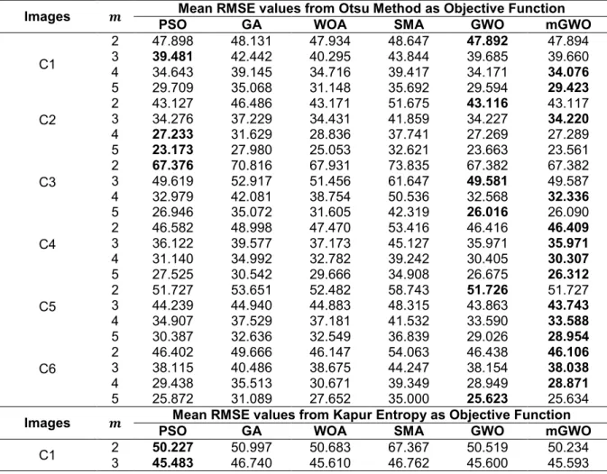
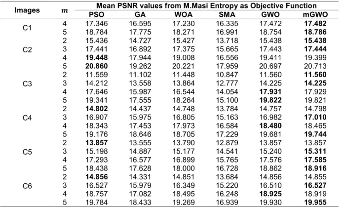
(3) The performance of the method implemented in this study was measured using qualitative and quantitative analysis using benchmark images from the USC- SIPI image database. Qualitative analysis was carried out by segmenting the six test images with each optimal threshold for each level. Quantitative analysis was carried out by calculating the fitness, RMSE, PSNR, SSIM, UQI, and CPU time values of each objective function.
(4) Hyperparameter tuning based on GridSearch is performed to obtain the optimal parameter combination of each SI method involved with the aim of maximizing the Otsu method.
(5) Statistical analysis using the Wilcoxon signed-rank test was used to test the significance of differences in the quantitative measurements of the GWO and mGWO methods against the benchmark method assigned to the test images.
(6) Comparing the results of the mGWO and GWO performance tests on grayscale images with other state-of-the-art methods in terms of fitness values and CPU Time (seconds).
MULTILEVEL THRESHOLDING FOR COLOR IMAGE SEGMENTATION
This section describes the definition of multilevel thresholding for mathematical image segmentation based on the Otsu, Kapur Entropy, and M.Masi Entropy methods.
Assume that there is an i-th 2D grayscale image as 𝐶𝑖𝑔𝑟𝑎𝑦 sized 𝑅 × 𝐾 with gray level 𝐺 = {0,1,2, … , 𝐿 − 1}. The R value represents the number of rows, while the K value represents the number of columns. So, an i-th RGB color image as 𝐶𝑖𝑅𝐺𝐵 can be defined as
a function vector [13] 𝑓⃗⃗ (𝑥, 𝑦): 𝑅 × 𝐾: → 𝐶𝑖 𝑖𝑟× 𝐶𝑖𝑔× 𝐶𝑖𝑏, such that:
𝐶𝑖𝑅𝐺𝐵= [𝑓⃗⃗ (𝑥, 𝑦)] = [𝐶𝑖 𝑖𝑟, 𝐶𝑖𝑔, 𝐶𝑖𝑏]
with 𝐶𝑖𝑟, 𝐶𝑖𝑔, 𝐶𝑖𝑏 each represents the red, green, and blue components (channels) of an image whose combinations can generate any displayable color [13]. Therefore, an RGB color image is a 3D array of color pixels with size 𝑅 × 𝐾 × 3 [13]. 𝐶𝑖𝑥 notation is used to show any channel (RGB or grayscale) of an i-th image.
Suppose 𝑁𝑖 is the total number of pixels in 𝐶𝑖𝑥 with 𝑛𝑗 is the number of occurrences of the jth gray level. Normalized histogram of 𝐶𝑖𝑥 is a probability distribution of each 𝑔 ∈ 𝐺. The probability that the jth gray level occurs at 𝐶𝑖𝑥 is defined according to Equation 1. The main objective of multilevel thresholding is to find a number of m optimal thresholds {𝑡1, 𝑡2, … , 𝑡𝑚} so split 𝐶𝑖𝑥 into the 𝑚 + 1 regions or segment that meet predetermined criteria or objective functions (Otsu Method, Kapur Entropy, or M.Masi Entropy). Suppose 𝑚 + 1 regions from
𝐶𝑖𝑥 is defined as 𝑊(𝑖)=
{𝑊0(𝑖), 𝑊1(𝑖), … , 𝑊𝑚(𝑖)} with the range of gray level values of the pixels contained in 𝑊𝑗(𝑖) is defined according to Equation 2. 𝑔(𝑥,𝑦) value in Equation 2 is the gray level of the pixels in the (𝑥, 𝑦) coordinates from a 2D image 𝐶𝑖𝑥.
𝑃𝑗(𝑖)= 𝑛𝑁𝑗
𝑖, (0 ≤ 𝑃𝑗(𝑖)≤ 1) ∧ (∑𝐿−1𝑘=0𝑃𝑘(𝑖)= 1)
( 1 ) 𝑊0(𝑖)= {𝑔(𝑥,𝑦)∈ 𝐶𝑖 | 0 ≤ 𝑔(𝑥,𝑦)≤
𝑡1− 1}
𝑊1(𝑖)= {𝑔(𝑥,𝑦)∈ 𝐶𝑖 | 𝑡1≤ 𝑔(𝑥,𝑦)≤ 𝑡2− 1}
𝑊2(𝑖)= {𝑔(𝑥,𝑦)∈ 𝐶𝑖 | 𝑡2≤ 𝑔(𝑥,𝑦)≤ 𝑡3− 1}
…
𝑊𝑚(𝑖)= {𝑔(𝑥,𝑦)∈ 𝐶𝑖 | 𝑡𝑚≤ 𝑔(𝑥,𝑦)≤ 𝐿 − 1}
( 2 )
Otsu Method
Suppose 𝐹𝑂𝑡𝑠𝑢(𝑡1, 𝑡2, … , 𝑡𝑚) is a function that accepts several m thresholds {𝑡1, 𝑡2, … , 𝑡𝑚} so that split 𝐶𝑖𝑥 into 𝑚 + 1 regions according to Otsu’s criteria. 𝐶𝑖𝑥 image can be segmented properly using a threshold {𝑡1, 𝑡2, … , 𝑡𝑚} when it produces the maximum 𝐹𝑂𝑡𝑠𝑢(𝑡1, 𝑡2, … , 𝑡𝑚) value among all the existing m thresholds combinations. The Otsu method maximizes the value between class variance according to Equation 3. 𝜎𝑗 value is calculated using Equation 4. 𝜔𝑗 value represents the sum of the probabilities of selecting pixels in the 𝑊𝑗(𝑖) region
Jurnal Nasional Pendidikan Teknik Informatika : JANAPATI | 307
which is calculated using Equation 5. 𝜇𝑗 value is the average pixel intensity value in the 𝑊𝑗(𝑖) region which is calculated using Equation 6. 𝜇𝑇
value is the average pixel intensity value in 𝐶𝑖𝑥 which is calculated using Equation 7.
𝐹𝑂𝑡𝑠𝑢(𝑡1, 𝑡2, … , 𝑡𝑚) = ∑𝑚 𝜎𝑗
𝑗=0 = 𝜎0+
𝜎1+ ⋯ + 𝜎𝑚 ( 3 )
𝜎0= 𝜔0(𝜇0− 𝜇𝑇)2 𝜎1= 𝜔1(𝜇1− 𝜇𝑇)2
…
𝜎𝑚= 𝜔𝑚(𝜇𝑚− 𝜇𝑇)2
( 4 ) 𝜔𝑗= ∑𝑡(𝑗+1)−1𝑃𝑧(𝑖)
𝑧=𝑡𝑗 ( 5 )
𝜇𝑗= ∑ 𝑗 × (𝑃𝜔𝑧(𝑖)
𝑧)
𝑡(𝑗+1)−1
𝑧=𝑡𝑗 ( 6 )
𝜇𝑇= ∑ (𝜔𝑚𝑗=0 𝑗𝜇𝑗) ( 7 )
Kapur Entropy
Suppose 𝐹𝐾𝑎𝑝𝑢𝑟(𝑡1, 𝑡2, … , 𝑡𝑚) is a function that accepts several m thresholds {𝑡1, 𝑡2, … , 𝑡𝑚} so that split the 𝐶𝑖𝑥 into 𝑚 + 1 regions according to Kapur Entropy criteria. 𝐶𝑖𝑥 image can be segmented properly using a threshold {𝑡1, 𝑡2, … , 𝑡𝑚} when it produces the maximum 𝐹𝐾𝑎𝑝𝑢𝑟(𝑡1, 𝑡2, … , 𝑡𝑚) value among all the existing m thresholds combinations. The Kapur Entropy maximizes the variance value in 𝑊(𝑖) by using the entropy value according to Equation 8. 𝐸𝑛𝑗 value is the entropy value of the 𝑊𝑗(𝑖) region which is calculated using Equation 9.
𝐹𝐾𝑎𝑝𝑢𝑟(𝑡1, 𝑡2, … , 𝑡𝑚) = ∑𝑚 𝐸𝑛𝑗
𝑗=0 =
𝐸𝑛0+ 𝐸𝑛1+ ⋯ + 𝐸𝑛𝑚 ( 8 )
𝐸𝑛0= − ∑ 𝑃𝑤𝑧(𝑖)
0 𝑡1−1
𝑧=0 𝑙𝑛 (𝑃𝑤𝑧(𝑖)
0) , 𝑤0=
∑𝑡1−1𝑃𝑧(𝑖)
𝑧=0
𝐸𝑛1= − ∑ 𝑃𝑤𝑧(𝑖)
1 𝑡2−1
𝑧=𝑡1 𝑙𝑛 (𝑃𝑤𝑧(𝑖)
1) , 𝑤1 =
∑𝑡𝑧=𝑡2−11𝑃𝑧(𝑖)
…
𝐸𝑛𝑚= − ∑ 𝑃𝑤𝑧(𝑖)
𝑚 𝐿−1𝑧=𝑡𝑚 𝑙𝑛 (𝑃𝑤𝑧(𝑖)
𝑚) , 𝑤𝑚=
∑𝐿−1𝑧=𝑡𝑚𝑃𝑧(𝑖)
( 9 )
M.Masi Entropy
Suppose 𝐹𝑀𝑎𝑠𝑖(𝑡1, 𝑡2, … , 𝑡𝑚) is a function that accepts several m thresholds {𝑡1, 𝑡2, … , 𝑡𝑚} so that split the 𝐶𝑖𝑥 into 𝑚 + 1 regions according to M.Masi Entropy criteria. 𝐶𝑖𝑥 image can be segmented properly using a threshold {𝑡1, 𝑡2, … , 𝑡𝑚} when it produces the maximum 𝐹𝑀𝑎𝑠𝑖(𝑡1, 𝑡2, … , 𝑡𝑚) value among all the existing m thresholds combinations. The M.Masi Entropy maximizes the variance value in 𝑊(𝑖) by using the entropy value according to Equation 10 [3].
𝑀𝑀𝐸𝑗 value is the M.Masi Entropy for 𝑊𝑗(𝑖)
which is calculated using Equation 11. 𝜑𝑗 value on 𝑀𝑀𝐸𝑗 calculation is calculated using Equation 12. The value of 𝛼 in Equation 11 can be determined through experiments with a value range of -1 to 3 intervals of 0.1 [3]. The value of 𝛼 < 1 has been proven to produce good and stable segmented image quality [3].
𝐹𝑀𝑎𝑠𝑖(𝑡1, 𝑡2, … , 𝑡𝑚) = ∑𝑚 𝑀𝑀𝐸𝑗
𝑗=0 =
𝑀𝑀𝐸0+ 𝑀𝑀𝐸1+ ⋯ + 𝑀𝑀𝐸𝑚 ( 10 ) 𝑀𝑀𝐸0= 𝑙𝑜𝑔(1− (1−𝛼) × 𝜑0)
(1−𝛼)
𝑀𝑀𝐸1= 𝑙𝑜𝑔(1− (1−𝛼) × 𝜑1)
(1−𝛼)
…
𝑀𝑀𝐸𝑚= 𝑙𝑜𝑔(1− (1−𝛼) × 𝜑𝑚)
(1−𝛼)
( 11 )
𝜑0= ∑ 𝑃𝑤𝑧(𝑖)
0 𝑡1−1
𝑧=0 𝑙𝑜𝑔 (𝑃𝑤𝑧(𝑖)
0) , 𝑤0=
∑𝑡1−1𝑃𝑧(𝑖)
𝑧=0
𝜑1= ∑ 𝑃𝑤𝑧(𝑖)
1 𝑡2−1
𝑧=𝑡1 𝑙𝑜𝑔 (𝑃𝑤𝑧(𝑖)
1) , 𝑤1=
∑𝑡2−1𝑃𝑧(𝑖) 𝑧=𝑡1
…
𝜑𝑚= ∑ 𝑃𝑤𝑧(𝑖)
𝑚
𝐿−1𝑧=𝑡𝑚 𝑙𝑜𝑔 (𝑃𝑤𝑧(𝑖)
𝑚) , 𝑤𝑚=
∑𝐿−1 𝑃𝑧(𝑖) 𝑧=𝑡𝑚
( 12 )
MATERIAL AND METHODS
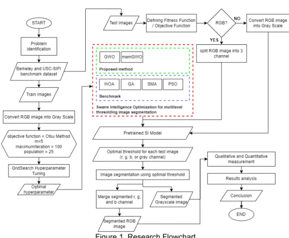
This section describes the steps taken to answer the research objectives along with the dataset used in this study as shown in Figure 1.
Benchmark Images
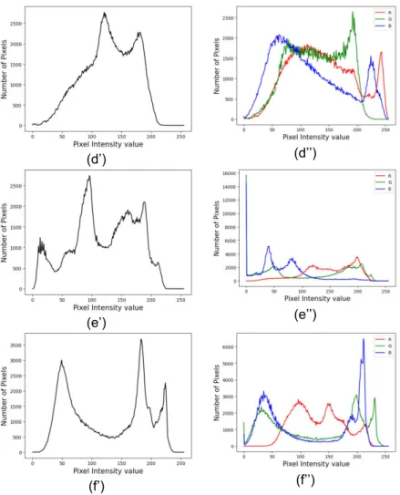
This study uses a standard benchmark dataset from the USC-SIPI image database and Berkeley BSDS 300. There are 10 images as training data and 6 images as test data. The training data is a combination of several image files selected from the train and test folders on the Berkeley BSDS 300 source. These files were chosen because they have multimodal histogram characteristics so that the optimal hyperparameters of each model can be selected objectively. The training data is used for the SI model development process for ML-ISP including the hyperparameter tuning process for each model. The test data that is used in this study are Airplane F16, Lena, Man, Mandrill (baboon), Peppers, and Sailboat on lake. The test data is used to evaluate the performance of the method used. Table 1 displays the names of the image files used as training data, while Figure 2 shows the pixel intensity histogram of the test data.
Grey Wolf Optimizer (GWO)
GWO is a method proposed by Mirjaili et al (2014) [22]. The GWO optimization method is inspired by social intelligence in hunting prey
Jurnal Nasional Pendidikan Teknik Informatika : JANAPATI | 308
and the social hierarchy of the gray wolf (Canis lupus) [14], [22], [24]. Gray wolves live in groups with 5 – 12 wolves in each group [14]. There are four levels or hierarchies in one group, namely alpha (𝛼), betha (𝛽), delta (𝛿), and omega (𝜔) wolves.
Alpha wolves are the highest level in this group whose job is to make decisions about hunting, where to sleep, when to wake up and so on. This wolf dominates the pack. The beta wolf is the second level after the alpha whose job is to help the alpha wolf make decisions and other group activities. The deltha wolf is the third level after betha whose duties are scout, caretaker, hunter, guard and scout. The omega wolf is the lowest level of this group which must submit to orders from all other dominant wolves [24].
Social hierarchy on GWO
The social hierarchy in a pack of gray wolves is divided into 𝛼, 𝛽, 𝛿, and 𝜔 wolves. In the mathematical modeling of the GWO method, the 𝛼, 𝛽, and 𝛿 wolves each represent the first, second and third best solutions [24]. The optimization process in this method is guided by the solutions produced by the three wolves, while the remaining 𝜔 wolves follow them [14].
Encircling of prey in GWO
During the hunt for prey, the gray
wolves surround their prey. This prey encirclement process is modeled mathematically according to Equations 13 and 14. The t-th iteration is expressed by the value (𝑡). The values of 𝐴 and 𝐶 are calculated using Equations 15 and 16, respectively. 𝑋⃗⃗⃗⃗⃗⃗⃗ 𝑝(𝑡) represents the position vector of the prey at iteration (𝑡), whereas 𝑋⃗⃗⃗⃗⃗⃗⃗ 𝑗(𝑡) represents the vector position of the gray wolf in iteration (𝑡). Vector 𝑎 decreases linearly in each iteration starting from 2 to 0 which is calculated using Equation 17 [21]. The maximum number of iterations is represented by 𝑇. The two random vectors in the interval [0,1] are represented by 𝑟⃗⃗⃗ 1 and 𝑟⃗⃗⃗ 2.
Figure 1. Research Flowchart
Table 1. List Files as Train Data File name Dimension
(pixel)
Color Space 101087.jpg 321 x 481
Gray 3096.jpg
481 x 321 106020.jpg
112082.jpg 113016.jpg 118035.jpg 119082.jpg 189003.jpg 231015.jpg 296059.jpg
Jurnal Nasional Pendidikan Teknik Informatika : JANAPATI | 309
The gray wolf moves in hypercubes or hyper- spheres around the best solution (𝛼 wolf) for a solution space of m dimension [14], [24].
𝐷⃗⃗ = |𝐶 ∙ 𝑋⃗⃗⃗⃗⃗⃗⃗ − 𝑋𝑝(𝑡) ⃗⃗⃗⃗⃗⃗⃗ |𝑗(𝑡) ( 13 ) 𝑋𝑗(𝑡+1)
⃗⃗⃗⃗⃗⃗⃗⃗⃗⃗⃗⃗ = 𝑋⃗⃗⃗⃗⃗⃗⃗ − 𝐴 ∙ 𝐷⃗⃗ 𝑝(𝑡) ( 14 ) 𝐴 = 2𝑎 ∙ 𝑟⃗⃗⃗ − 𝑎 1 ( 15 )
𝐶 = 2 ∙ 𝑟⃗⃗⃗ 2 ( 16 )
𝑎 = 2 (1 − 𝑇𝑡) ( 17 )
Hunting process in GWO
The 𝛼, 𝛽, and 𝛿 wolves guide the hunting process of all wolves in a group. These three wolves are assumed to have better knowledge of the potential location of a prey (optimal solution). Hence all the other wolves updated their positions based on the information on the three wolves. The mathematical model for the prey hunting process is according to Equations 18 and 19. The position vectors of the 𝛼, 𝛽, and 𝛿 wolves in (𝑡) iteration are
represented by 𝑋⃗⃗⃗⃗⃗⃗⃗ 𝛼(𝑡), 𝑋⃗⃗⃗⃗⃗⃗⃗ 𝛽(𝑡), and 𝑋⃗⃗⃗⃗⃗⃗⃗ 𝛿(𝑡) respectively.
Vektor 𝐴⃗⃗⃗ dan 𝑖 𝐶⃗⃗⃗ are calculated using Equations 𝑖
15 and 16 with different sets of random numbers, respectively. The position vector of each gray wolf is updated using Equation 20.
𝐷𝛼
⃗⃗⃗⃗⃗ = |𝐶⃗⃗⃗⃗ ∙ 𝑋1 ⃗⃗⃗⃗⃗⃗⃗ − 𝑋𝛼(𝑡) ⃗⃗⃗⃗⃗⃗⃗ |𝑗(𝑡) 𝐷𝛽
⃗⃗⃗⃗ = |𝐶⃗⃗⃗⃗ ∙ 𝑋2 ⃗⃗⃗⃗⃗⃗⃗ − 𝑋𝛽(𝑡) ⃗⃗⃗⃗⃗⃗⃗ |𝑗(𝑡) 𝐷𝛿
⃗⃗⃗⃗ = |𝐶⃗⃗⃗⃗ ∙ 𝑋3 ⃗⃗⃗⃗⃗⃗⃗ − 𝑋𝛿(𝑡) ⃗⃗⃗⃗⃗⃗⃗ |𝑗(𝑡)
( 18 )
𝑋1(𝑡)
⃗⃗⃗⃗⃗⃗⃗ = 𝑋⃗⃗⃗⃗⃗⃗⃗ − 𝐴𝛼(𝑡) ⃗⃗⃗⃗ ∙ 𝐷1 ⃗⃗⃗⃗⃗ 𝛼
𝑋2(𝑡)
⃗⃗⃗⃗⃗⃗⃗ = 𝑋⃗⃗⃗⃗⃗⃗⃗ − 𝐴𝛽(𝑡) ⃗⃗⃗⃗ ∙ 𝐷2 ⃗⃗⃗⃗ 𝛽 𝑋3(𝑡)
⃗⃗⃗⃗⃗⃗⃗ = 𝑋⃗⃗⃗⃗⃗⃗⃗ − 𝐴𝛿(𝑡) ⃗⃗⃗⃗ ∙ 𝐷3 ⃗⃗⃗⃗ 𝛿
( 19 )
𝑋𝑗(𝑡+1)
⃗⃗⃗⃗⃗⃗⃗⃗⃗⃗⃗⃗ = 𝑋⃗⃗⃗⃗⃗⃗⃗⃗ 1(𝑡)+ 𝑋⃗⃗⃗⃗⃗⃗⃗⃗ 23(𝑡)+ 𝑋⃗⃗⃗⃗⃗⃗⃗⃗ 3(𝑡) ( 20 ) Attacking the prey (exploitation) in GWO
Vector 𝐴 and vector 𝐶 in the above equation are used to store the exploration and
(a’) (a’’)
(b’) (b’’)
(c’) (c’’)
Figure 2. The benchmark (RGB) image data used for evaluating the performance of the method was obtained from the USC-SIPI image database. Each image in (a) – (f) has a size of 512 x 512 pixels
along with their respective grayscale histograms (a') – (f') and RGB histograms (a'') – (f'') with (a) Airplane F-16, (b) Lena, (c) Man, (d) Mandrill (Baboon), (e) Peppers, and (f) Sailboat on lake.
Jurnal Nasional Pendidikan Teknik Informatika : JANAPATI | 310
exploitation abilities of wolves [21]. The process of hunting prey from wolves is completed by attacking prey by wolves. This process is modeled by reducing the value of the vector 𝑎 in the range 2 to 0 during the iteration process.
The fluctuation range of 𝐴 will decrease if 𝑎 is also decrease. When |𝐴⃗⃗⃗⃗⃗⃗⃗ | < 1(𝑡) and/or |𝐶⃗⃗⃗⃗⃗⃗⃗ | <(𝑡) 1, then a pack of wolves attacks the prey [14], [21]. When |𝐴⃗⃗⃗⃗⃗⃗⃗ | > 1(𝑡) and/or |𝐶⃗⃗⃗⃗⃗⃗⃗ | > 1(𝑡) , then the new search area explored by the pack of wolves can avoid being stuck at the local optimum [14], [21]. Exploration and exploitation operators are balanced by using a value transition from vector 𝑎 at each (𝑡) iteration.
GWO for solving ML-ISP
The GWO algorithm is used in this study to find the optimal threshold value (represented by the position of the wolf) at the mth level so that it can be used to segment images with a maximum of 𝑚 + 1 regions. One wolf in GWO represents a solution for which you want to find the optimal value. The input of this process is the histogram of the image to be
segmented, while the output of this process is the optimal position vector of the wolf as 𝑋∗ which represents the optimal threshold value.
The positional vector representation of each i-th wolf is written as 𝑋⃗⃗⃗ which is initialized 𝑖 according to Equation 22. The total number of wolves initialized is written as N. The value 𝑥(𝑖,𝑗)∈ 𝑋⃗⃗⃗⃗⃗⃗⃗ 𝑖(𝑡) is the threshold value represented by the gray level of an image. At the beginning of the iteration (𝑡 = 0), the fitness of all wolves is calculated with a predetermined objective function, namely using the Otsu method, Kapur Entropy, or M.Masi Entropy respectively with Equations 3, 8 or 10. Three wolves with fitness values optimal is then defined as 𝑋⃗⃗⃗⃗⃗⃗⃗ 𝛼(0),⃗⃗⃗⃗⃗⃗⃗ 𝑋𝛽(0), dan 𝑋𝛿(0)
⃗⃗⃗⃗⃗⃗⃗ . For each iteration during a predetermined maximum iteration T, each wolf updates its position taking into account the positions of the three 𝛼, 𝛽, and 𝛿 wolves using Equation 20.
Before updating the positions, vector 𝐴⃗⃗⃗ , vector 𝑖
𝐶𝑖
⃗⃗⃗ , and vector 𝑎 is calculated using Equations 15, 16, and 17 respectively.
(d’) (d’’)
(e’) (e’’)
(f’) (f’’)
Figure 2. (Continued).
Jurnal Nasional Pendidikan Teknik Informatika : JANAPATI | 311
The updated vector 𝑋⃗⃗⃗⃗⃗⃗⃗ 𝑖(𝑡) can be outside the constraints of ML-ISP when the value𝑥(𝑖,𝑗) is outside the range of gray level G. Therefore, Equation 21 is used to adjust 𝑋⃗⃗⃗⃗⃗⃗⃗ 𝑖(𝑡) to be in the problem solution space in this study. Then, the fitness value of each i-th wolf is written as 𝐹𝑖𝑡(𝑋⃗⃗⃗ )𝑖 which is calculated in the same way as when 𝑡 =0. The position vectors of the wolves 𝛼, 𝛽, and 𝛿 at each iteration 𝑋⃗⃗⃗⃗⃗⃗⃗ 𝛼(𝑡),𝑋⃗⃗⃗⃗⃗⃗⃗ 𝛽(𝑡), and 𝑋⃗⃗⃗⃗⃗⃗⃗ 𝛿(𝑡) are updated based on the three wolves with optimal fitness.
𝑋𝑖(0)
⃗⃗⃗⃗⃗⃗⃗ = [𝑥(𝑖,1), 𝑥(𝑖,2), … , 𝑥(𝑖,𝑚)], (𝑖 = 1,2, … , 𝑁) ∧ (0 < 𝑥(𝑖,1)…< 𝑥(𝑖,𝑚)<
𝐿) 𝑥(𝑖,𝑗)= 𝑟𝑎𝑛𝑑𝐼𝑛𝑡(0, (𝐿 − 1))
( 22 )
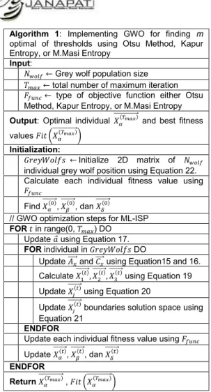
GWO Pseudocode for solving ML-ISP
Pseudocode of the GWO Algorithm to solve ML-ISP is presented as in Figure 3.
Memory-based Grey Wolf Optimizer (mGWO)
𝑋𝑗(𝑡+1)
⃗⃗⃗⃗⃗⃗⃗⃗⃗⃗⃗⃗ = {𝐿 − 𝑟𝑜𝑢𝑛𝑑(𝑟𝑎𝑛𝑑𝑜𝑚(0,1) ∗ 𝑟𝑎𝑛𝑑𝑜𝑚𝐼𝑛𝑡𝑒𝑔𝑒𝑟(0, 𝐿)), (𝑥(𝑖,𝑗)) > 𝐿 0, (𝑥(𝑖,𝑗)) < 0
𝑥(𝑖,𝑗), 𝑜𝑡ℎ𝑒𝑟𝑤𝑖𝑠𝑒
, ∀𝑥(𝑖,𝑗)∈𝑋⃗⃗⃗⃗⃗⃗⃗⃗⃗⃗⃗⃗⃗⃗ 𝑗(𝑡+1) ( 21 ) Algorithm 1: Implementing GWO for finding m
optimal of thresholds using Otsu Method, Kapur Entropy, or M.Masi Entropy
Input:
𝑁𝑤𝑜𝑙𝑓← Grey wolf population size 𝑇𝑚𝑎𝑥← total number of maximum iteration 𝐹𝑓𝑢𝑛𝑐← type of objective function either Otsu Method, Kapur Entropy, or M.Masi Entropy Output: Optimal individual 𝑋⃗⃗⃗⃗⃗⃗⃗⃗⃗⃗⃗⃗⃗⃗ 𝛼(𝑇𝑚𝑎𝑥) and best fitness values 𝐹𝑖𝑡 (𝑋⃗⃗⃗⃗⃗⃗⃗⃗⃗⃗⃗⃗⃗⃗ )𝛼(𝑇𝑚𝑎𝑥)
Initialization:
𝐺𝑟𝑒𝑦𝑊𝑜𝑙𝑓𝑠 ← Initialize 2D matrix of 𝑁𝑤𝑜𝑙𝑓
individual grey wolf position using Equation 22.
Calculate each individual fitness value using 𝐹𝑓𝑢𝑛𝑐
Find 𝑋⃗⃗⃗⃗⃗⃗⃗ 𝛼(0), 𝑋⃗⃗⃗⃗⃗⃗⃗ 𝛽(0), dan 𝑋⃗⃗⃗⃗⃗⃗⃗ 𝛿(0)
// GWO optimization steps for ML-ISP FOR 𝑡 in range(0, 𝑇𝑚𝑎𝑥) DO
Update 𝑎 using Equation 17.
FOR individual in 𝐺𝑟𝑒𝑦𝑊𝑜𝑙𝑓𝑠 DO
Update 𝐴⃗⃗⃗⃗ and 𝑥 𝐶⃗⃗⃗⃗ using Equation15 and 16. 𝑥
Calculate 𝑋⃗⃗⃗⃗⃗⃗⃗ ,𝑋1(𝑡)⃗⃗⃗⃗⃗⃗⃗ ,𝑋2(𝑡)⃗⃗⃗⃗⃗⃗⃗ 3(𝑡) using Equation 19 Update 𝑋⃗⃗⃗⃗⃗⃗⃗ 𝑗(𝑡) using Equation 20
Update 𝑋⃗⃗⃗⃗⃗⃗⃗ 𝑗(𝑡) boundaries solution space using Equation 21
ENDFOR
Update each individual fitness value using 𝐹𝑓𝑢𝑛𝑐
Update 𝑋⃗⃗⃗⃗⃗⃗⃗ 𝛼(𝑡), 𝑋⃗⃗⃗⃗⃗⃗⃗ 𝛽(𝑡), dan 𝑋⃗⃗⃗⃗⃗⃗⃗ 𝛿(𝑡) ENDFOR
Return 𝑋⃗⃗⃗⃗⃗⃗⃗⃗⃗⃗⃗⃗⃗⃗ 𝛼(𝑇𝑚𝑎𝑥) , 𝐹𝑖𝑡 (𝑋⃗⃗⃗⃗⃗⃗⃗⃗⃗⃗⃗⃗⃗⃗ )𝛼(𝑇𝑚𝑎𝑥)
Figure 3. GWO pseudocode for ML-ISP
Jurnal Nasional Pendidikan Teknik Informatika : JANAPATI | 312
The GWO proposed by Mirjaili et al (2014) [22] is considered vulnerable to being stuck at the optimum local value when used to solve multimodal problems because the update process from 𝑋⃗⃗⃗⃗⃗⃗⃗ 𝑖(𝑡) only depends on three leader wolves [21]. The wolf pack will find it difficult to get out of the optimum locale when the three wolves are trapped in the optimum locale because they only depend on them [21].
Therefore, Gupta and Deep (2020) [21]
proposed an update process of 𝑋⃗⃗⃗⃗⃗⃗⃗ 𝑖(𝑡) integrating the best track record of each wolf with the positions of the three lead wolves. It aims with the intention of involving the best knowledge of each wolf in the process of exploring the solution space to guide the wolf pack to explore or move into a promising solution space and not get stuck at local optimum values [21].
All the symbols in this section are the same as those in the previous section. In mGWO, the encircling prey process is updated using Equation 23 [21]. Vector 𝑋⃗⃗⃗⃗⃗⃗⃗⃗⃗⃗⃗⃗⃗⃗⃗⃗⃗ 𝑝𝑏𝑒𝑠𝑡 (𝑗)(𝑡) is the
best position vector stored in the memory of the j-th wolf in the (𝑡) iteration. The process of hunting prey involving the three 𝛼, 𝛽, and 𝛿 wolves is updated using Equation 24 [21].
Equation 24 [21] is proposed with the intention of imitating the thought that each wolf may have information on prey and use it to explore and retrace the surrounding wolf area using 𝑋𝑝𝑏𝑒𝑠𝑡 (𝑗)(𝑡)
⃗⃗⃗⃗⃗⃗⃗⃗⃗⃗⃗⃗⃗⃗⃗⃗⃗ .
Algorithm 2: Implementing mGWO for finding m optimal of thresholds using Otsu Method, Kapur Entropy, or M.Masi Entropy
Input:
𝑁𝑤𝑜𝑙𝑓← Grey wolf population size 𝑇𝑚𝑎𝑥← total number of maximum iteration 𝐶𝑅 ← crossover rate
𝐹𝑓𝑢𝑛𝑐← type of objective function either Otsu Method, Kapur Entropy, or M.Masi Entropy Output: Optimal individual 𝑋⃗⃗⃗⃗⃗⃗⃗⃗⃗⃗⃗⃗⃗⃗ 𝛼(𝑇𝑚𝑎𝑥) and best fitness values 𝐹𝑖𝑡 (𝑋⃗⃗⃗⃗⃗⃗⃗⃗⃗⃗⃗⃗⃗⃗ )𝛼(𝑇𝑚𝑎𝑥)
Initialization:
𝐺𝑟𝑒𝑦𝑊𝑜𝑙𝑓𝑠 ← Initialize 2D matrix of 𝑁𝑤𝑜𝑙𝑓
individual grey wolf position using Equation 22.
𝑚𝑒𝑚𝑜𝑟𝑦𝐺𝑟𝑒𝑦𝑊𝑜𝑙𝑓𝑠 ← Save the initial best position of 𝐺𝑟𝑒𝑦𝑊𝑜𝑙𝑓𝑠
𝑝𝐵𝑒𝑠𝑡𝐹𝑖𝑡𝑛𝑒𝑠𝑠 ← Calculate each individual fitness value using 𝐹𝑓𝑢𝑛𝑐
Find 𝑋⃗⃗⃗⃗⃗⃗⃗ 𝛼(0), 𝑋⃗⃗⃗⃗⃗⃗⃗ 𝛽(0), dan 𝑋⃗⃗⃗⃗⃗⃗⃗ 𝛿(0)
// mGWO optimization steps for ML-ISP FOR 𝑡 in range(0, 𝑇𝑚𝑎𝑥) DO
Update 𝑎 and 𝑘(𝑡) using Equation 17 and 26.
FOR individual in 𝐺𝑟𝑒𝑦𝑊𝑜𝑙𝑓𝑠 DO
Update 𝐴⃗⃗⃗⃗ and 𝑥 𝐶⃗⃗⃗⃗ using Equation15 and 16. 𝑥 IF 𝑟𝑎𝑛𝑑(0,1) < 𝐶𝑅 DO
Calculate 𝑋⃗⃗⃗⃗⃗⃗⃗ ,𝑋1(𝑡)⃗⃗⃗⃗⃗⃗⃗ ,𝑋2(𝑡)⃗⃗⃗⃗⃗⃗⃗ 3(𝑡) using Equation 19
Update 𝑋⃗⃗⃗⃗⃗⃗⃗ 𝑗(𝑡) using Equation 24 ELSE
Find two of 𝑋⃗⃗⃗⃗⃗⃗⃗⃗⃗⃗⃗⃗⃗⃗⃗⃗ 𝑟𝑎𝑛𝑑 (𝑗)(𝑡) randomly Update 𝑋⃗⃗⃗⃗⃗⃗⃗ 𝑗(𝑡) using Equation 25 ENDIF
Update 𝑋⃗⃗⃗⃗⃗⃗⃗ 𝑗(𝑡) boundaries solution space using Equation 21
ENDFOR
Update each individual fitness value using 𝐹𝑓𝑢𝑛𝑐
FOR 𝑖 = 1,2, … 𝑁𝑤𝑜𝑙𝑓 DO
IF 𝐹𝑖𝑡 (𝑋⃗⃗⃗⃗⃗⃗⃗ )𝑖(𝑡)
>
𝑝𝐵𝑒𝑠𝑡𝐹𝑖𝑡𝑛𝑒𝑠𝑠 (𝑖) DO 𝑚𝑒𝑚𝑜𝑟𝑦𝐺𝑟𝑒𝑦𝑊𝑜𝑙𝑓𝑠(𝑖)(𝑡)= 𝑋⃗⃗⃗⃗⃗⃗⃗ 𝑖(𝑡) 𝑝𝐵𝑒𝑠𝑡𝐹𝑖𝑡𝑛𝑒𝑠𝑠(𝑖)= 𝐹𝑖𝑡 (𝑋⃗⃗⃗⃗⃗⃗⃗ )𝑖(𝑡)ENDIF ENDFOR
Update 𝑋⃗⃗⃗⃗⃗⃗⃗ 𝛼(𝑡), 𝑋⃗⃗⃗⃗⃗⃗⃗ 𝛽(𝑡), dan 𝑋⃗⃗⃗⃗⃗⃗⃗ 𝛿(𝑡) ENDFOR
Return 𝑋⃗⃗⃗⃗⃗⃗⃗⃗⃗⃗⃗⃗⃗⃗ 𝛼(𝑇𝑚𝑎𝑥) , 𝐹𝑖𝑡 (𝑋⃗⃗⃗⃗⃗⃗⃗⃗⃗⃗⃗⃗⃗⃗ )𝛼(𝑇𝑚𝑎𝑥)
Figure 4. mGWO pseudocode for ML-ISP Algorithm 3: Segmenting process of 𝐶𝑖 using 𝑚
optimal threshold
Input: 2D pixels array of image 𝐶𝑖, 𝑚 optimal threshold T
Output: segmented image 𝑆𝑖
Initialization:
row ← row shape of 𝐶𝑖
col ← col shape of 𝐶𝑖
regionThres ← dictionary()
flatCi ← convert 2D of 𝐶𝑖 into 1D array // Get lower and upper bound for each threshold boundaries
FOR idx in range(0, m+1) DO IF idx is 0 DO
bb_thres ← 0 ba_thres ←𝑇𝑖𝑑𝑥− 1 ELIF idx is m DO
bb_thres ←𝑇𝑖𝑑𝑥−1
ba_thres ←𝐿 − 2 ELSE
bb_thres ←𝑇𝑖𝑑𝑥−1
ba_thres ←𝑇𝑖𝑑𝑥− 1 𝑟𝑒𝑔𝑖𝑜𝑛𝑇ℎ𝑟𝑒𝑠(𝑖𝑑𝑥)← [𝑏𝑏, 𝑏𝑎]
ENDIF ENDFOR
// Convert each pixel values of 𝐶𝑖 to correspondent bb and ba
FOR idx, pixel in enumerate(flatCi) DO FOR regionId, interval in regionThres DO
IF pixel ≥ 𝑖𝑛𝑡𝑒𝑟𝑣𝑎𝑙(0)AND pixel ≤ 𝑖𝑛𝑡𝑒𝑟𝑣𝑎𝑙(1) DO
𝑓𝑙𝑎𝑡𝐶𝑖(𝑖𝑑𝑥) ← 𝑖𝑛𝑡𝑒𝑟𝑣𝑎𝑙(1)+ 1 ENDIF
ENDFOR ENDFOR
𝑆𝑖← reshape flatCi to row and col dimension Return 𝑆𝑖
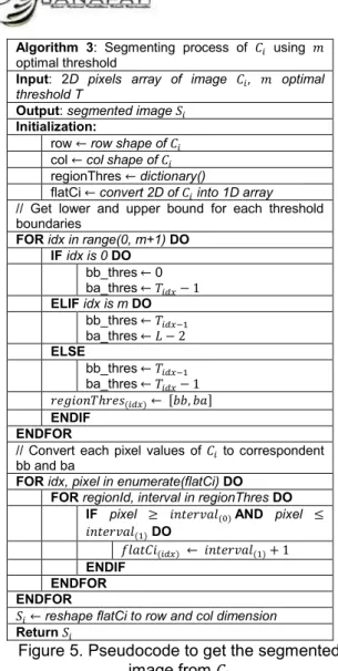
Figure 5. Pseudocode to get the segmented image from 𝐶𝑖
Jurnal Nasional Pendidikan Teknik Informatika : JANAPATI | 313
In Equation 25, two wolf positions are chosen at random which are written as 𝑋⃗⃗⃗⃗⃗⃗⃗⃗⃗⃗⃗⃗⃗⃗⃗⃗ 𝑟𝑎𝑛𝑑 (𝑗)(𝑡+1) . The 𝑘 value is the scale factor used to adjust the effect of subtracting the two position vectors.
The value of 𝑘 decreases linearly from 1 to 0 in each iteration which is updated using Equation 26. The crossover process is then carried out in the update stage 𝑋⃗⃗⃗⃗⃗⃗⃗⃗⃗⃗⃗⃗ 𝑗(𝑡+1). The process combines information from the three best wolves with each individual wolf according to Equation 27. The crossover probability value is written as CR and random numbers in the range 0 to 1 with a uniform distribution are written as 𝑟.
𝑋𝑗(𝑡+1)
⃗⃗⃗⃗⃗⃗⃗⃗⃗⃗⃗⃗ = 𝑋⃗⃗⃗⃗⃗⃗⃗ − 𝐴 ∙ 𝐷⃗⃗ = 𝑋𝑝(𝑡) ⃗⃗⃗⃗⃗⃗⃗ − 𝐴 ∙𝑝(𝑡)
|𝐶 ∙ 𝑋⃗⃗⃗⃗⃗⃗⃗ − 𝑋𝑝(𝑡) ⃗⃗⃗⃗⃗⃗⃗⃗⃗⃗⃗⃗⃗⃗⃗⃗⃗ |𝑝𝑏𝑒𝑠𝑡 (𝑗)(𝑡) ( 23 ) 𝑍𝑗(𝑡+1)
⃗⃗⃗⃗⃗⃗⃗⃗⃗⃗⃗ = 𝑆⃗⃗⃗⃗⃗⃗⃗⃗ 1(𝑡)+ 𝑆⃗⃗⃗⃗⃗⃗⃗⃗ 2(𝑡)3 + 𝑆⃗⃗⃗⃗⃗⃗⃗⃗ 3(𝑡) 𝑆1(𝑡)
⃗⃗⃗⃗⃗⃗ = 𝑋⃗⃗⃗⃗⃗⃗⃗ − 𝐴𝛼(𝑡) ⃗⃗⃗⃗ ∙ |𝐶 1 1∙ 𝑋⃗⃗⃗⃗⃗⃗⃗ −𝛼(𝑡) 𝑋⃗⃗⃗⃗⃗⃗⃗⃗⃗⃗⃗⃗⃗⃗⃗⃗⃗ |𝑝𝑏𝑒𝑠𝑡 (𝑗)(𝑡)
𝑆2(𝑡)
⃗⃗⃗⃗⃗⃗ = 𝑋⃗⃗⃗⃗⃗⃗⃗ − 𝐴𝛽(𝑡) ⃗⃗⃗⃗ ∙ |𝐶 2 2∙ 𝑋⃗⃗⃗⃗⃗⃗⃗ −𝛽(𝑡) 𝑋⃗⃗⃗⃗⃗⃗⃗⃗⃗⃗⃗⃗⃗⃗⃗⃗⃗ |𝑝𝑏𝑒𝑠𝑡 (𝑗)(𝑡)
𝑆3(𝑡)
⃗⃗⃗⃗⃗⃗ = 𝑋⃗⃗⃗⃗⃗⃗⃗ − 𝐴𝛿(𝑡) ⃗⃗⃗⃗ ∙ |𝐶 3 3∙ 𝑋⃗⃗⃗⃗⃗⃗⃗ −𝛿(𝑡) 𝑋⃗⃗⃗⃗⃗⃗⃗⃗⃗⃗⃗⃗⃗⃗⃗⃗⃗ |𝑝𝑏𝑒𝑠𝑡 (𝑗)(𝑡)
( 24 )
𝑃𝑗(𝑡+1)
⃗⃗⃗⃗⃗⃗⃗⃗⃗⃗⃗ = 𝑋⃗⃗⃗⃗⃗⃗⃗⃗⃗⃗⃗⃗⃗⃗⃗⃗⃗ + 𝑘𝑝𝑏𝑒𝑠𝑡 (𝑗)(𝑡) (𝑡+1)∙
(𝑋⃗⃗⃗⃗⃗⃗⃗⃗⃗⃗⃗⃗⃗⃗⃗⃗ − 𝑋𝑟𝑎𝑛𝑑 (𝑗)(𝑡+1) ⃗⃗⃗⃗⃗⃗⃗⃗⃗⃗⃗⃗⃗⃗⃗⃗ ) 𝑟𝑎𝑛𝑑 (𝑗)(𝑡+1) ( 25 )
𝑘(𝑡) =
(
1 − 𝑇𝑡)
( 26 )𝑋𝑗(𝑡+1)
⃗⃗⃗⃗⃗⃗⃗⃗⃗⃗⃗⃗ = { 𝑍⃗⃗⃗⃗⃗⃗⃗⃗⃗⃗⃗ ,𝑟 < 𝐶𝑅𝑗(𝑡+1) 𝑃𝑗(𝑡+1)
⃗⃗⃗⃗⃗⃗⃗⃗⃗⃗⃗ ,𝑜𝑡ℎ𝑒𝑟𝑤𝑖𝑠𝑒 ( 27 ) mGWO pseudocode for solving ML-ISP
Pseudocode of the mGWO Algorithm to solve ML-ISP is presented as in Figure 4.
Image Segmentation with Optimal Threshold
Each channel in the 𝐶𝑖𝑥 test image is then segmented using the optimal threshold value that has been obtained from the SI method-based optimization process. The pseudocode in Figure 5 is used to divide the 𝐶𝑖𝑥image into 𝑚 + 1 regions using optimal {𝑡1, 𝑡2, … , 𝑡𝑚}. The 𝐶𝑖𝑥 image that has been segmented with the optimal 𝑚 threshold is denoted as 𝑆𝑖𝑅𝐺𝐵 for RGB color images and 𝑆𝑖𝑔𝑟𝑎𝑦 for grayscale images.
𝑆𝑖𝑅𝐺𝐵 is obtained by combining the segmentation results from 𝐶𝑖𝑟, 𝐶𝑖𝑔, and 𝐶𝑖𝑏. Assume thresholding levels for each channel r, g, and b in the RGB image, namely 𝑚𝑟, 𝑚𝑔, and 𝑚𝑏. The SI method is implemented to obtain the optimal threshold value for each channel. Each optimal threshold value is used to segment each channel using the pseudocode in Figure 5. The segmented image for each channel is denoted as 𝑆𝑖𝑟, 𝑆𝑖𝑔, and 𝑆𝑖𝑏 such that:
𝑆𝑖𝑅𝐺𝐵= [𝑆𝑖𝑟, 𝑆𝑖𝑔, 𝑆𝑖𝑏]
Therefore, 𝑆𝑖𝑅𝐺𝐵 has the most 𝑚𝑟 × 𝑚𝑔 × 𝑚𝑏
color levels and fewer than 𝐶𝑖𝑅𝐺𝐵[13].
EXPERIMENTS
Experiments in this study were conducted to measure the performance stability of the GWO and mGWO methods to solve ML- ISP using three different objective functions, namely the Otsu method, Kapur Entropy, and M.Masi Entropy. As a comparison, another standard IS optimization method is involved, namely the Genetic Algorithm (GA) [20], [25]– [28], Particle Swarm Optimization (PSO) [1], [9], [13], Whale Optimization Algorithm (WOA) [8], [12], [18], and Slime Mould Algorithm (SMA) [8], [23]. All comparison methods used are standard SI methods and not variants or optimized versions of these methods.
For the comparison to be fair, all methods used in this study use optimization stopping criteria, namely the maximum number of iterations is 100, with a population of 25 solutions, and the number of trials for each method is 30 [18]. The number of thresholds evaluated for each image in the test data is 2, 3, 4, and 5 as in previous studies [3], [4], [6]–[8], [14], [15], [18].
All methods are programmed and evaluated using the Python3.10 programming language which is implemented in the device environment Windows 10 – 64 bit, Intel Core i7- 8565U CPU @1.80GHz and 8GB of RAM.
GridSearch Hyperparameter Tuning
The hyperparameter tuning process was carried out to obtain the optimal parameter combination for each method (as shown in Table 2) used in this study. It aims to obtain a fair comparison of performance metrics for each method at the evaluation stage. This study uses the GridSearch scheme for the hyperparameter tuning process. The GridSearch method looks for all possible combinations of each hyperparameter value and then gets the parameter combination that gives the most optimal results based on the predefined metrics.