Nonlinear Dynamics of Nanoscale Systems

(1)

Thesis by

Nathan Oken Hodas

In Partial Fulfillment of the Requirements for the Degree of

Doctor of Philosophy

California Institute of Technology Pasadena, California

2011

(Defended May 6, 2011)

(2)

c 2011 Nathan Oken Hodas

(3)

“The Sun is a mass of incandescent gas...”

—Why Does the Sun Shine? by They Might by Giants

“The Sun is a miasma of incandencent plasma. The Sun’s not simply made of gas...

That thesis has been rendered invalid!”

—Why Does the Sun Really Shine? by They Might be Giants

(4)

Acknowledgements

I am honored to thank so many people for helping and guiding me over the past years.

I learned a great deal in my previous life in Hideo Mabuchi’s lab. Mike Armen and Andy Berglund made great squash partners as well as great tutors, enthusiastically teaching me all about optics and electronics. I really appreciate Ramon van Handel’s patience with my questions about Markov processes and the Fokker-Planck equation.

Kevin McHale and Asa Hopkins were great office- and benchmates. I also want to thank Tony Miller, John Au, John Stockton, Ben Lev, Nicole Czakon, Gopal Sarma, Orion Crisafulli, and Joe Kerckhoff. The quantitative finance seminar with Luc Bouten and Tim McGarvey was fun and a welcome diversion when I was trying to get over the hump of my third and fourth year, plus I now understand the Ito calculus. Of course, the other member of the Mabuchi lab to remain at Caltech, Sheri Stoll, was both a friend and a resource, and without her I would not know about Li¯o, the boy who loves giant squid.

A tip from Andy started a collaboration with Kris Helmerson at NIST. It was there I really learned about single molecule microscopy. I thank Kris for hosting me in Maryland for those many weeks. I enjoyed worked closely with Jauyang Tong and Ana Jofre, with whom I spent many hours in a darkened tent trying to catch droplets

(5)

of water with a laserbeam. Many thanks to Rani Kishore for working with me to advance the hydrosome project, doing much of the DNA wet work, and teaching me the best ways to prepare pristine samples. It was a shame we could never get things to work completely before Hideo left for Stanford, but my time at NIST also taught me that cutting edge research requires squashing gremlin after gremlin. Otherwise, it would have been done already! I have many thanks for Hideo for supporting me and encouraging me, and I know I have missed out on a lot by not following the lab to Stanford. That said, I have no regrets for staying at Caltech.

I have many people to thank in my second life at Caltech. The members of the Marcus lab, past and present, were great companions at our Friday lunches, Zhaoyan Zhu, Wei-Chen Chen, Yousung Jung, Evans Boney, Maksym Kryvohuz, Nima Ghaderi, and Yun-Hua Hong. I also want to thank Jau Tang for help with the GFPmut2 project and Yanting Wang for doing the simulations for the SFG work. I want to extend extra thanks to Evans and Nima for sharing so many great conversa- tions and for productive collaborations. It is hard to express adequate appreciation for the mentorship and advising from Rudy. Every minute was enlightening and infor- mative, and I was lucky to be able to work with someone so dedicated to his students and supportive of my interests.

In the Fraser lab, I also have many people to thank. Aura Keeter was indispensable for helping me find my way around the lab and helping with maxi-preps and getting machines to work. I extend similar appreciation to Mary Flowers, the lab mom, Kristy Hilands, the former lab administrator, and Pat Anguiano, Scott’s admin. I

(6)

am indebted to the help from Christie Canaria, who shared so many reagents and protocols with me. I have special thanks for Thai Truong for helping me with the microscopes and many helpful discussions. I also thank Jeff Fingler for our last minute attempts to use OCT to measure the refractive index of zebrafish. It was worth a try. Thanks to Jelena Culic-Viskota for tirelessly working to perfect the SHG nanoparticles. WIthout Andres Collazo, I would not have had access to the House Ear Institute’s Zeiss 710, and he was great to talk to while sitting in that dark, cold room. Thanks to my officemates, Mat Barnet, Cambrian Liu, and, recently, Danielle Bower. I would not have even had an office if it weren’t for the generosity of Larry Wade, who knew exactly what I was going through when we were both struggling to get things to work. To my closest collaborators, Bill Dempsey and Laki Pantazis, you both taught me a great deal, and I would not be graduating now if it weren’t for your help and advice. You have also been good friends, and I was lucky to find such great partners. I also thank the other members of the lab for their support, including Le Trinh, Luca Caneparo, Roee Amit, Max Ezin, Alana Dixon, Greg Reeves, Frederique Ruf, David Huss, David Koos, and Dave Wu. Of course, I extend my deep thanks to Scott Fraser, whose advice and insight proved vital over and over. Without your great sense for experimental design, I would still be shooting lasers at globs of barium titanate, and I am honored that you were willing to support me after Hideo left.

There were many people outside the lab who helped me reach this point. Edgardo Garcia was the right person at the right time to help me, and I’m lucky to have him as a friend. Best of luck in San Jose. Of course, all of my fellow RAs helped me

(7)

successfully navigate the world of the Caltech undergraduate housing system. Also, many thanks to Dean Barbara Green, Sue Chiarchiaro, Geoff Blake, and Tim Chang for helping us overcome so many challenges with the students. Ruddock House was our home for three years, and it was an amazing time. We laughed, we cried, and we learned a lot about life. It was the second half of my life at Caltech, outside research, and it was very fulfilling.

I am lucky to have such a loving family to help me through. As a new parent, I am now doubly aware how nurturing and supportive my parents have been at every step of my life. I don’t know how they dealt with me, but I am lucky to have them. Of course, it’s easy to thank little Leo. There is nothing like coming home to his bright face to help me relax and recharge, and my productivity significantly increased after he joined us. He even literally inspired a section of my thesis, and he is duly noted in that chapter. Last, it is hard to overstate the help I got from my wife and best friend, Jenn. From helping me purify GFPmut2 to supporting our family while I went into hermit mode to write my thesis, she was there every step of the way; and I am lucky to have such a caring companion, and I look forward to spending many future happy years together. This work is dedicated to you. Love, Sq.

(8)

Abstract

This work builds theoretical tools to better understand nanoscale systems, and it explores experimental techniques to probe nanoscale dynamics using nonlinear optical microscopy. In both the theory and experiment, this work harnesses nonlinearity to explore new boundaries in the ongoing attempts to understand the amazing world that is much smaller than we can see. In particular, the first part of this work proves the upper-bounds on the number and quality of oscillations when the system in question is homogeneously driven and has discrete states, a common way of describing nanoscale motors and chemical systems, although it has application to networked systems in general. The consequences of this limit are explored in the context of chemical clocks and limit cycles. This leads to the analysis of spontaneous oscillations in GFPmut2, where we postulate that the oscillations must be due to coordinated rearrangement of the beta-barrel. Next, we utilize nonlinear optics to probe the constituent structures of zebrafish muscle. By comparing experimental observations with computational models, we show how second harmonic generation differs from fluorescence for confocal imaging. We use the wavelength dependence of the second harmonic generation conversion efficiency to extract information about the microscopic organization of muscle fibers, using the coherent nature of second

(9)

harmonic generation as an analytical probe. Finally, existing experiments have used a related technique, sum-frequency generation, to directly probe the dynamics of free OH bonds at the water-vapor boundary. Using molecular dynamic simulations of the water surface and by designating surface-sensitive free OH bonds on the water surface, many aspects of the sum-frequency generation measurements were calculated and compared with those inferred from experiment. The method utilizes results available from independent IR and Raman experiments to obtain some of the needed quantities, rather than calculating them ab initio. The results provide insight into the microscopic dynamics at the air-water interface and have useful application in the field of on-water catalysis.

(10)

Contents

Acknowledgements iv

Abstract viii

1 Introduction 1

2 Oscillations on Networks 6

2.1 The Limits of Oscillations in Overdamped Systems . . . 8

2.2 The Limits on Oscillations . . . 10

2.3 Oscillations in Macrostates: Chemical Clocks . . . 13

2.4 Oscillations in Green Fluorescent Protein GFPmut2 . . . 18

2.4.1 Limit Cycles . . . 21

2.4.2 Loop Dynamics . . . 30

2.5 Conclusion . . . 36

3 Endogenous Second Harmonic Generation in Zebrafish 39 3.1 Structure of Muscle . . . 42

3.1.1 Muscle Construction . . . 42

3.1.2 Optical Properties of Muscle . . . 47

(11)

3.2 Methods for Measuring Second Harmonic Generation . . . 52

3.3 Discussion . . . 59

3.3.1 Representative Images . . . 59

3.3.2 Wavelength-Dependent SHG . . . 63

4 Theory of Second Harmonic Generation from Zebrafish Muscle 74 4.1 Foundations of Nonlinear Optics . . . 74

4.2 SHG Phase-Matching with Focused Light . . . 79

4.2.1 The Paraxial Approximation of the Wave Equation . . . 80

4.2.2 SHG from Periodic Media . . . 82

4.3 Explaining Patterns in Muscle Structure . . . 90

4.4 Wavelength Dependence of SHG . . . 95

4.4.1 Wavelength Dependence Due to Myofibril Packing . . . 99

4.4.2 Wavelength Dependence Due to Collection Efficiency . . . 102

5 Microscopic Structure and Dynamics of Air/Water Interface by Computer Simulations and Comparison with Sum-Frequency Gen- eration Experiments 107 5.1 Methods . . . 109

5.2 Results and Discussion . . . 122

Bibliography 129

(12)

List of Figures

2.1 The regionR_N in the complex plane contains all possible eigenvalues of

N-dimensional stochastic matrices with unit spectral radius . . . 12

2.2 Oscillations as a function of system size . . . 14

2.3 The effect of system size on macrostate oscillations . . . 14

2.4 Ribbon representation of GFP . . . 22

2.5 The local neighborhood of the GFP chromophore . . . 23

2.6 When the chromophore is anionic its excess charge draws its tightly coupled neighbors into alignment with the chromophore. When neutral, the amino acids are now free to preferentially align with their neighbors, increasing the structural rigidity of the β-barrel. . . 27

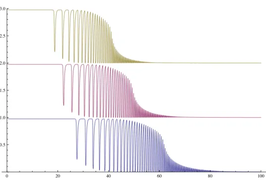
2.7 Oscillations produced by two-variable model . . . 28

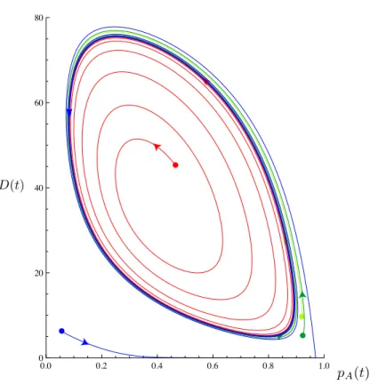
2.8 Phase-space dynamics of GFPmut2 denaturing . . . 31

2.9 Time-dependent rates create a transition from a static system to a limit cycle. . . 32

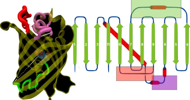
2.10 Illustration of secondary and tertiary structure of GFP . . . 33

2.11 Baby Leo’s toy, the bead maze, is an example of linear motion producing a periodic signal. . . 36

(13)

3.1 Sagittal section of zebrafish 36 hours post fertilization, with composite brightfield . . . 41 3.2 Anatomical planes. Zebrafish are oriented laterally, meaning the sagittal

plane is parallel to the ground and perpendicular to the laser. . . 42 3.3 Label-free image of fixed zebrafish embryo, sagittal section. . . 43 3.4 Second harmonic generation from muscle and collagen . . . 44 3.5 (a) A multiscale illustration of muscle organization, and (b) a cartoon

of the process of muscle contraction. . . 46 3.6 TEM micrographs of myofibril crosssection, showing hexagonal packing

of myosin and actin. . . 47 3.7 TEM images of muscle fibers . . . 48 3.8 Reflection of 850 nm laser pulses indicates the optical density of the

zebrafish transverse section . . . 50 3.9 Using experimentally measured refraction index data from porcine mus-

cle [120] (total internal reflection), we determine the refractive index across the entire spectrum. Points are experimental data, line is fit by eq. (3.1). . . 52 3.10 Each element of the imaging pathway has different wavelength depen-

dent transmission or sensitivity. . . 55 3.11 Fluorescent debris from the zebrafish were used to measure point spread

functions at 790 nm, 850 nm, and 890 nm, using 25x 0.8 NA . . . 56

(14)

3.12 An image of second harmonic generation from morphant zebrafish, optically sectioned along the sagittal plane. Lesions are evidenced by the circular outlines of luminescence. . . 57 3.13 Epithelial cells accumulate damage over a 2 minute exposure to 820 nm

Ti-Sapphire laser pulses . . . 58 3.14 High maginfication view of discrete structure of myofibrils. . . 60 3.15 Second harmonic generation from wildtype. . . 61 3.16 Inset shows magnified view of herringbone or “vernier” pattern from a

7 day post-fertilization zebrafish. . . 62 3.17 Transgenic fish were used to visualize the interface between myofibril

SHG and fluorescent-protein labeled membranes and nuclei . . . 67 3.18 Multiple views of membrane-labeled wildtype zebrafish . . . 68 3.19 Second harmonic generation from zebrafish morphant muscle. . . 69 3.20 Comparison of SHG from sagittal sections between (a) wildtype and (b)

morphant. . . 70 3.21 The wavelength dependent SHG detected from a single sagittal plane of

5-day old zebrafish . . . 71 3.22 Normalized intensity spectrum density map of points from figure 3.21 of

low-intensity background points. . . 72 3.23 The wavelength dependent SHG detected from a single coronal plane of

5-day old morphany zebrafish . . . 73

(15)

4.1 Second harmonic generation production efficiency depends on the magnitude of the phase-matching, ∆k, determined by eq. (4.7). Absent perfect phase-matching, corresponding to ∆k = 0, SHG can only be produced across a distance constrained by ∆k∆x <2π. . . 79 4.2 With a focused beam, the conversion efficiency is very sensitive to the

magnitude and sign of the phase-matching, ∆k, as well as the width of the medium, z_f −z₀. b= 0.5 . . . 83 4.3 Theoretical calculations illustrate the qualitative difference between SHG

and two-photon fluorescence . . . 92 4.4 Tilting the laser causes the SHG doublets to disappear . . . 96 4.5 The nonlinear susceptibility of muscle, χ⁽²⁾(ω), based on Miller’s rule. . 97 4.6 Plot of SHG susceptibility map. Here, p= 2. . . 101 4.7 `_cas a function of wavelength for the refractive index defined in Eq 3.1.

All units are µm. . . 101 4.8 Fit of eq. (4.37) using the quasi-phase-matching structure in eq. (4.36),

with p= 5µm. The experimental data are from figure 3.21. Thex-axis is wavelength in nanometers, and the y-axis normalized intensity. . . . 102 4.9 SHG emission has angular dependence . . . 103 4.10 The wavelength dependent SHG may also be due to the variation of the

size of the laser focus. Here, the SHG active region was constrained to a box extending 5.2b along the z-axis and 1.9w₀ along the x- and y-axis. 104

5.1 The simulated water/vacuum interface . . . 126

(16)

5.2 Probability density of the cosine of the tilt angle with respect to the surface normal . . . 127 5.3 Correlation functions of free OH bonds produced by simulation, using

three different snapshot times, 1 , 10 , and 100 fs. . . 128

(17)

List of Tables

5.1 Average number of free surface OH bonds, hN_OHi, and average orientation angle, hθ_OHi, of free surface OH bonds calculated from three MD simulations with different snapshot time intervals . . . 125 5.2 Results of fitting the calculated spectrum to a Lorentzian and correcting

for experimental width. . . 125

(18)

Chapter 1 Introduction

The nanoscale is the spatial regime at least 10 times larger than atoms and simple molecules, yet also 10 times too small to be resolved by the unaided human eye. Such small things are often readily disturbed by the constant jostling of their air and liquid environments. A grandfather clock that is 50 nm tall will not tick, no matter how precisely it is machined. A bacteria does not swim by paddling through water like a fish, instead it moves by spinning a flagella. Making things smaller can make them different. Gold, when broken down into 10 nanometer crystals, transforms in color from the familiar shiny metal into a deep red, and silver turns yellow. Hence, nan- otechnology is exciting not just because we can make big things smaller but because we can make new things.

A crystal composed of thousands or millions of atoms may have completely differ- ently properties from its isolated constituent atoms and may also be different from a larger version of the same crystals. At first, this would be no surprise to someone like a baker, who transforms unpalatable flour, salt, baking soda, fat, and sugar into deli- cious doughnuts. But, making a doughnut is a series of chemical reactions, while the changes in size-dependent properties occur spontaneously. A better analogy would be

(19)

making a doughnut by cutting it out of a pizza, and suddenly it was sweet and savory, or by squeezing two pieces of rye bread together and ending up with tasty dessert.

These metaphors are drawn from examples in this thesis, where we explore how the optical properties of water at the water-vapor boundary are different from those in the liquid bulk. We prove that making a system larger may allow it to oscillate longer and more predictably. Finally, we consider how the microscopic arrangement of protein fibers in muscle interact nonlinearly with laser light, yet a different arrangement of the same proteins on the nanoscale would make such a nonlinear interaction impossible. We use this information to learn more about the organization of muscles on the microscopic level.

Nanoscale systems often contain a limited number of relevant states,¹ and we often want to do something useful with those states, such as operate a motor protein or convert light into electricity. These require highly correlated dynamics that persist in time. Unfortunately, damping by the environment, due to buffeting by solvent molecules, tends to prevent oscillatory dynamics which might be necessary for successful operation of nano-machines or chemical systems. The second law of ther- modynamics implies that no macroscopic system may oscillate indefinitely without consuming energy, so dissipation is not surprising prima facie. Yet, the maximum number of possible oscillations and the coherent quality of these oscillations remain unknown, until now. The first part of this work proves the upper-bounds on the number and quality of such oscillations when the system in question is homogeneously

1An obvious exception to this rule would be living biological systems. They are both nanoscale and have a large number of relevant states, but we try our best to focus on only the most essential parts.

(20)

driven and has discrete states. In a closed system, the maximum number of oscillations is bounded by the number of states. In open systems, the system size bounds the quality factor of oscillation, which is a figure of merit for the predictability of recurring behavior. This work also explores how the quality factor of macrostate oscillations, such as would be observed in chemical reactions, are bounded by the smallest loop in the reaction network, not the size of the entire system. The consequences of this limit are explored in the context of chemical clocks and limit cycles.

This leads to the analysis of spontaneous oscillations in denatured GFPmut2, where, using these principles, we identify the oscillation mechanism to be the coordinated rearrangement of the hydrogen bond network of the β-barrel. We further calculate that the oscillations are touched off by one of the major loops adjoining theβ-barrel, which provide a verifiable means to control the oscillation period.

To optically probe probing nanoscale systems of biological relevance with conven- tional techniques often requires one to use a focused laser to achieve highest possible signal contrast and resolution. Fluorescent labels in the sample absorb light from the laser and emit a photon with less energy. The detection of the low-energy photon then indicates the presence of the labeled object of interest. Unfortunately, the diffraction limit leads to a fundamental bound of the resolving power of the conven- tional microscope. To achieve higher resolution, we utilize nonlinear optics to probe the constituent structures of zebrafish muscle. In this case, nonlinearity is a tool for extracting additional information. Because the myosin fibers are asymmetric on the nanoscale, they have the ability to fuse two photons into one, a process known as sec-

(21)

ond harmonic generation. Instead of looking for a photon with less energy than the incoming laser, as with fluorescence, we try to detect photons with twice the energy of the incoming light. Second harmonic generation (SHG) based images can be very similar to fluorescence but with up to twice the resolution. Additionally, because light produced via second harmonic generation is coherent, while fluorescence is incoher- ent, the images have subtle yet significant differences, which we explore and explain.

We use the wavelength dependence of the second harmonic generation conversion efficiency to extract information about the microscopic organization of muscle fibers, using the coherent nature of second harmonic generation as an analytical probe.

Second harmonic generation only occurs when the underlying material is asymmetric on the nanometer scale, and this is always the case at the boundary between two different materials. Existing experiments have used technique related to SHG, called sum-frequency generation (SFG), to directly probe the dynamics of free OH bonds at the water-vapor boundary. Using molecular dynamics simulations of the water surface, and by designating surface-sensitive free OH bonds on the water surface, we attempt to computationally reproduce the SFG experiment. The corresponding SFG susceptibility measurements were calculated and compared with those inferred from experiment. The method utilizes results available from independent IR and Raman experiments to obtain some of the needed quantities, rather than calculating them ab initio, allowing us to focus on the components of the water dynamics that best capture the observed SFG signature. We determine that the rotational dynamics, with a small quantum correction, are sufficient to produce the observed SFG signal.

(22)

The results provide insight into the microscopic dynamics at the air-water interface, and has useful application in the field of on-water catalysis.

To properly establish the path through all of these topics, I note my role in each. The first chapter is work which I have undertaken myself. The research on the GFPmut2 oscillations was directed by Rudy Marcus and advised by Scott Fraser, but the work is primarily my own. The work on zebrafish muscle was a close collaboration with Bill Dempsey, under the direction of Scott Fraser. Bill prepared all of the zebrafish for imaging, injected the morphants, and produced the transgenic fish. I imaged the fish and conducted the computations and theory. The SFG project was directed by Rudy Marcus, and it has since been published [1] and an addendum as been posted with necessary updates.² Yanting Wang produced the MD simulations.

Yousung Jung and Professor Marcus spearheaded the project. I helped construct the theory with Professor Marcus and process the simulation data. Without this help and guidance from all of these individuals, especially Professors Marcus and Fraser, I certainly would not have much to report, nor would I know nearly as much as I do now.

2http://www.rsc.org/suppdata/cp/c0/c0cp02745f/addition.htm

(23)

Chapter 2

Oscillations on Networks

To better understand how to build, design, and operate nanoscale machines, we have to understand more about what makes dynamics on the smallest scales different from dynamics we observe in our everyday lives. By dynamics, we refer to the dis- placements, oscillations, and momentum transformations that give rise to observable behavior. Although popular science is full of interesting discussions of how the world of quantum mechanics leads to wonderful and nonintuitive dynamics, this is only part of the story of why small is different. Classical dynamics, “the science of the 19^th century,” plays a central role. The reason, in short, is “scaling.”

Consider an object in a fluid medium. It is subject to buffeting by molecules of the medium, which deliver kicks that knock the mass off-course, but conservation of momentum also causes the same molecules to sap momentum from any directed motion the body may possess. Newton’s law states that F =ma, but the total force on the object will be a combination of endogenous forces (which are those forces still acting on the body even in a vacuum) and the buffeting and damping forces from the viscous medium. If the endogenous forces are extensive, meaning they are proportional to the size of the object, they scale asR³, whereR is the effective radius

(24)

of the object. In contrast, the fluid medium acts on the surface area of the object, so the forces from the bath causing buffeting and damping scale as R². Thus, the ratio of the endogenous forces, which are the forces we would rely on to do useful work, to the bath forces, which impart noise, scale asR. The smaller an object gets, the smaller the endogenous forces become in relation to the bath forces. At a critical length scale, which would depend on the precise forces involved and the nature of the immersion medium, the buffeting and damping by the bath would completely swamp the object’s ability to do persistent work. This scaling has been well explored in fluid mechanics via a number of ratios to understand the balance of various factors [2].

Reynolds number, in particular, captures the change in viscous dynamics relative to inertial dynamics as length scales shrink. It is defined as Re = V L/ν, where V is the velocity of the object, L is a characteristic length scale, and ν is the kinematic viscosity. When Re is small, inertial forces are overwhelmed by viscous forces, and any directed motion is rapidly quenched.

Small objects inherently live in the world of small Re. In the low Reynolds number regime, dynamic motion such as oscillations cannot be sustained. This chapter will explore ways to create oscillatory behavior in the low Reynolds number regime. It has direct application to the design of nanoscale machines and the operation of proteins within the body.

(25)

2.1 The Limits of Oscillations in Overdamped Sys- tems

Oscillations are ubiquitous. We celebrate them and attempt to harness them. Nat- urally, this interest drives us to study them. There has been no shortage of analysis of the simple harmonic oscillator in all of its variations, but much of the periodic- ity around us is not equivalent to a mass on a spring. For example, the beating heart is driven by molecular motors which exist in the low-Reynolds number regime, where viscous damping overwhelms inertial forces. For these molecular constituents, buffeting by solvent molecules prevents coherent oscillations from persisting on a timescale longer than the mean time between collisions, which is on order picoseconds [3]. Despite this, we observe the coordination of overdamped components to produce periodic behavior [4]. Studying this coordination on a problem-by-problem basis has uncovered some conceptual principles to designing oscillatory behavior in the overdamped regime, but few truly fundamental laws exist [5, 6, 7, 8, 9]. This work bounds the performance of all discrete-state over-damped oscillatory systems, providing a new look at the necessary conditions for creating coherent oscillations in overdamped systems.¹

When the energy landscape of an overdamped system can be divided into distinct basins of attraction with barriers higher than k_BT, the system will tend to reach a local equilibrium within a basin of the energy landscape before fluctuations stochas-

1We all possess an intuitive comfort with oscillations, but we have to formalize this notion for our analysis. To separate coherent oscillations from random fluctuations, we demand that oscillations be predictable and have a characteristic timescale. Predictability implies that the autocorrelation of a signal will have distinct peaks or troughs corresponding to the period of the oscillations.

(26)

tically drive it over a barrier into a neighboring basin. Under these conditions, it is common and appropriate to model each basin as a distinct state, with a fixed rate of transitioning from one state to another [10, 11, 12]. These systems are finite state first-order Markov processes² and can be modeled by the master equation:

dp_i(t) dt =

N

X

j

T_ijp_j(t)−

N

X

j6=i

T_ijp_i(t), (2.1)

whereTij is the transition rate from statej to statei. For introductions to the master equation and its numerous physical applications see [13, 14]. We will assume that all rates are time-independent, meaning no external factors change the rates (but does not necessarily mean that the system is closed). We also make the assumption that T is an irreducible matrix, enforcing the trivial condition that we are not modeling multiple mutually isolated systems. Finally, we assume that the systems conserve probability, which can always be enforced by adding states to the system to represent sinks. The solution to eq. (2.1) isp(t) = exp(Tt)p(0), where Tis matrix notation for T_ij, T_ii =−P

j6=iT_ji and p(t) is vector notation for p_j(t) [15]. Systems represented by the master equation are completely described by the transition rate matrix, T, and the initial conditions p(0). The complete solution is

p(t) =X

j

v_je^λ^j^t V_j⁻¹·p(0) +a_j(t)

, (2.2)

where v_j is the j^th eigenvector and V⁻¹ is the inverse of the matrix of eigenvec-

2This means we exclude systems with high degrees of quantum coherence or those that are underdamped and therefore inertial. The systems in question completely thermalizes before changing states. Without loss of generality, we will only describe the probability of occupying a given state.

(27)

tors.³ Hence, characterizing the properties of T also characterizes the dynamics of the system [16, 17, 13]. Because the time dynamics of individual modes are ultimately determined by the eigenvalues of T (see eq. (2.2)), we will be concerned with these eigenvalues and how they relate to oscillations. We first explore these eigenvalues and prove how they constrain the possible oscillations to be fewer than the number of states in the system. Second, I provide examples of these limits by exploring the quality of oscillations in a hypothetical stochastic clock, showing how both microscopic oscillations and macrostates are constrained by the number of states in the system. I conclude by proposing some experiments which may cast direct light onto the physical realization of these bounds on oscillations.

2.2 The Limits on Oscillations

To understand the oscillations in the system represented by T, we consider the relative contributions of different eigenmodes. From the Perron-Frobenius theorem, all eigenvalues of T have nonpositive real parts, so all but the λ = 0 equilibrium mode decay away. Eigenvectors with nonzero imaginary eigenvalues oscillate in magnitude as they decay. As we see in eq. (2.2), after a time (Reλ_i)⁻¹, mode i’s contribution top(t) will have substantially diminished. If there is an imaginary part toλ_i, before decaying modei will oscillate|Imλ_i/Reλ_i|times. Because each oscillatory mode will have a resonance independent of the other modes, the overall quality of oscillations

3Dennery, P. & Kryzwicki, A.Mathematics for Physicists, Dover 1996.

(28)

is given by :

Q= 1 2max

i |Imλi/Reλi|. (2.3)

In closed systems, Q is the upper bound on the number of oscillations. In an open and homogeneously driven system, Qdescribes the coherence of those oscillations, in analogy to the quality-factor of harmonic oscillators. This work establishes upper- bounds on Q by showing the eigenvalues of T only exist in specific regions of the complex plane.

Karpelevich’s Theorem, as clarified by Ito [18, 19], states that all possible eigenvalues of anN-dimensional stochastic matrix with unit spectral radius (max_i|λ_i|= 1) are contained in a bounded region, which we call R_N, on the complex plane, shown in figure 2.1. R_N intersects the unit circle at points exp(2πia/b), where a and b are relatively prime and 0 ≤ a < b ≤ N. The curve connecting points z = e^2πia¹^/b¹ and z =e^2πia²^/b² is described by the parametric equation

z^b²(z^b1−s)^bN/b¹^c=z^b¹^bN/b¹^c(1−s)^bN/b¹^c, (2.4)

wheresruns over the interval [0,1] andbx/ycis the integer floor ofx/y. For example, the curve that connects z = 1, corresponding to (a₁ = 0, b₁ = N), with z = e^2πi/N (a₂ = 1, b₂ =N) is z(s) = (e^2πi/N−1)s+ 1.

The rate matrix from eq. (2.1), T, is not a stochastic matrix. To preserve probability, the sum of each columns of T is zero, and the diagonal elements are ≤ 0.⁴

4This may be obtained by lettingpi= (1,0,0, . . .), substitutingpi into eq. (2.1), and solving for the conditionP

ipi= 0.

(29)

0.5

0.0

-0.5 1.0

1.0 -1.0 -0.5 0.0 0.5

-1.0

Im

Re N=3 N=4 N=5

R N

Figure 2.1: The regionR_N contains all possible eigenvalues ofN-dimensional stochastic matrices with unit spectral radius. Region R_N₊₁ contains R_N. This region is symmetric to the real axis and circumscribed by the unit circle. The curves defining each region are given by eq. (2.4), due to Karpelevich’s Theorem.

To transform T into a stochastic matrix, denoted T⁰, divide T by the sum of its largest diagonal element and largest eigenvalue, and add the identity matrix. This transformation allows us to write the eigenvalues ofT⁰ in terms of the eigenvalues of T:

λ⁰_i = λ_i

max_j|T_jj|+ max_j|λ_i| + 1. (2.5) Because the most positive eigenvalues of the original T are 0 and all others have negative real parts, the most positive eigenvalue ofT⁰ is 1. This unique normalization technique ensures all other eigenvalues are less than 1 and fit within the region R_N on the complex plane. Therefore, all of the eigenvalues ofT, will fit within the region (max_i|T_ii|+ max_i|λ_i|)×(R_N −1), where these operations on R_N denote scaling and translation, respectively. Within this transformed region, the maximum number of

(30)

oscillations will be produced by eigenvalues on the line λ∝(e^±2πi/N −1), giving

Q_max = 1 2

sin(2π/N) cos(2π/N)−1

= 1

2cot(π/N)< N

2π. (2.6)

We can further refine the limit in eq. (2.6) using a result from Kellogg and Stephens [20], giving

Q_max= 1 2cot π

`cyc

< `_cyc

2π , (2.7)

where `_cyc is the longest cycle in the system.

Up to this point in our proof, we have restricted ourselves to systems without any degeneracy in the eigenvalues of T. With degeneracy, as shown in eq. (2.2) , the time dependence of eigenvectorj may pick up an extra polynomial factor, a_j(t), with degree less than the degeneracy of λ_j, which is always less than N −1. Fortuitous balancing of coefficients could allow a p^th-order polynomial to add an additional p/2 oscillations. Examining eq. (2.2), we see that the total maximum oscillation quality can be

Q_max< `cyc

π + N −1

2 < N, (2.8)

where the second term is strictly due to degeneracy⁵

2.3 Oscillations in Macrostates: Chemical Clocks

Oscillations which consist of cycles on the discrete state-space are only possible when the system in question violates detailed balance [17], which would be the case in a

5Such degeneracy will usually emerge only in hypothetical systems where rates balance perfectly.

(31)

1 2 3 4

1 2

N=2 N=4

(A) (B)

N = 80 40 20 10

Spectral Density

5

frequency (arb. units)

Figure 2.2: (a) When the energy landscape has barriers much larger than k_BT, the system will spend most of its time in the minima of the environment. Approximating the continuous landscape by discrete states gives the familiar master equation kinetics.

Here we document two examples of systems with unidirectional transition rates. This cyclical system produces the maximumQfor any given N. (b) As shown in eq. (2.6), a system with only two states cannot coherently oscillate. It produces only random jumps. As the number of states in the unidirectional cycle increases (in the same family as shown in (a)), oscillations become more coherent and more persistent. The spectral density of the unidirectional cycle shows a distinct peak which becomes sharper as N increases. The transition rates have been normalized by the number of states. The Q of the systems are, from bottom to top: 0.75,1.46,3.09,6.40,12.7, obtained by fitting Lorentzian functions to the peaks.

(B) (A)

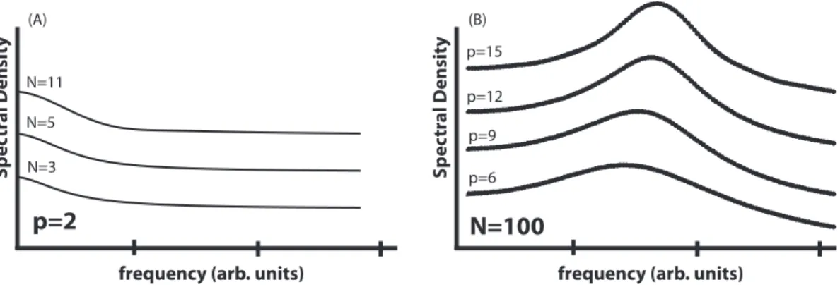
p=6 p=9 p=12 p=15

p=2 N=100

Spectral Density

frequency (arb. units)

Spectral Density

frequency (arb. units) N=3

N=5 N=11

Figure 2.3: Although the linear set of states given by eq. (2.9) does not have any imaginary eigenvalues, macrostates can oscillate. Macrostates are defined as hAi = PN

i A^p_ip_i(t). In this case, A^p_i = {1 if mod_pi = 0; 0 otherwise}. (a) Dynamics for different values of N for fixed p= 2 (inset) Identical dynamics, but with scaled rates so expected traversal times are the same. (b) Increasing p increases the number and coherence of oscillations given fixed N = 61, demonstrating the limit in eq. (2.7).

(32)

system which is driven. Otherwise, conservation of energy prevents the system from completing a cycle without encountering significant energy barriers. The microstates of the system, represented by the instantaneous values of p(t), would not show any oscillatory dynamics or peaks in the spectral density, shown in figure 2.2(a). On the other hand, oscillations in macrostates, which are the linear superpositions hA(t)i= P

iA_ip_i(t), do not require the underlying microstates to oscillate. The microstate probabilities only need to evolve such that hA(t)i oscillates. For example, consider a hypothetical chemical clock⁶ described by a cycle of states [22, 10]

s₁ → · · · →s_N →s₁. (2.9)

If the clock advances each time the cycle is traversed, adding states to the cycle improves the quality of the clock, as shown in Fig 2.2(b). A more abstract implemen- tation could be to consider a clock cycle and a fuel reservoir. We define that the clock consumes 1 unit of fuel during the transition from s_N back to s₁, so the cycle is an open system. This accounting method, in effect, unrolls the cycle into a linear chain of microstates enumerated by the dyad{f, s_i}, wheref is the amount of fuel remaining.

Whenf is effectively infinite, the dynamics of the open cycle and the linear chain are equivalent. As the system moves from one state to another, we count time by keeping track of the evolution of the macrostate denotedA(t). The macrostate of the clock is hA(t)i = P

i,fA_ip(f, s_i, t) = P

iA_ihp(s_i, t)i. Therefore, the quality of oscillations in

6The oscillating chemical clock is distinct from the traditional “clock reaction,” where an au- tocatalytic reaction causes a sudden one-time change in state on a distinct timescale, such as the iodate-bisulphite system [21].

(33)

the infinite linear chain is bounded by Q_s, regardless of the precise amount of fuel.

WhenAi ={1 if mod2i= 0; 0 otherwise},as shown in figure 2.3(a), the total number of states, N does not effect the quality of the clock. However, if we changeA_i to

A^p_i ={1 if mod_pi= 0; 0 otherwise},

figure 2.3(b) shows increasing oscillation in hA(t)iwith increasing p. That is, adding more states to the clock directly increases its accuracy.

Texts exploring chemical oscillations state that nonlinearity is a requirement for oscillations. In fact, nonlinearity is a shorthand for describing extremely large systems [13]. Under conditions of detailed balance, systems must consume some sort of fuel to sustain oscillations. If we consider the fuel-free states as being an abstract engine with N states, the combined engine-fuel system will be in one of the N different states and have f units of fuel remaining. Therefore, a fuel reservoir can allow a total number of oscillations ≈ f N/π. eq. (2.8) implies that the number of inherently unique states, absent fuel consumption, will constrain the possible regularity of reciprocal motion [10]. Thus, the quality of oscillations appears to be bounded by the smallest irreducible cycle in the system, although this is not proven. That is, the topology of the network is inherently related to the ability of the system to sustain oscillations, and this will be explored in future work.

Similarly, if the system is driven by oscillations in multiple parameters or species, we can again parameterize the state of the system based on the population of each component. However, most chemical dynamics are modeled using continuous vari-

(34)

ables, not discrete numbers of states. The microscopic description of the system, comprised of a discrete number of states, is connected to the continuous mass-action approximation of chemical dynamics by a system size expansion described by Van Kampen [13]. Take, as an example, the multidimensional oscillating chemical reaction called the Brusselator. By expanding the mass-action Brusselator into a discrete state-space, the system size-expansion parameter determines the length of the largest cycle [23, 24]. Indeed, multiple authors have observed that the quality of the Brussela- tor limit cycle scales with system size, consistent with this work [23, 22, 25, 26, 27, 24].

This observation is not merely coincidence, but a fundamental efficiency limit of the master equation.

This efficiency limit of oscillations has obvious implications on how well a high- dimensional system can be numerically approximated by a smaller system. The approximation will only be successful if the relevant eigenvalues of the larger system lie within the allowed region of the smaller system. However, the inverse stochastic eigenvalue problem has not yet been solved, so we cannot knowa priori if a stochastic matrix exists for a given set of eigenvalues, even if they all reside within the allowed region [28]. This fact prevents us from constructing the opposite bounds, the conditions for a minimum number of oscillations. Hopefully, future results will further constrain the present bounds, and we may gain deeper insight into the necessary conditions for creating oscillations.

The bounds on oscillations can play a key role in interpreting experimental observations by determining a minimum number of underlying states. For example,

(35)

the oscillation of fluorescence wavelength in fluorescent protein GFPmut2 remains unexplained [29, 30, 31]. After application of a denaturant, the ionic state of the fluorophore can switch up to Q ∼ 50 times with high regularity, observed as oscillations in the emission wavelength [29]. Because eq. (2.7) bounds the number of states involved in the oscillation to be at least 3 times larger thanQ, this predicts that the oscillations are driven by large-scale rearrangement of the numerous hydrogen bonds in the β-barrel, not merely exchange between the few amino acids directly connected to the fluorophore. If the protein were to be mutated to alter the number of bonds in the β-barrel, we predict that we should see a corresponding alteration in the number and quality of observed oscillations.

2.4 Oscillations in Green Fluorescent Protein GF- Pmut2

In a series of recent experiments, a mutant of Green Fluorescent Protein, GFPmut2, was encapsulated in silica gel and observed under denaturing conditions [32, 33, 31].

Ordinarily, when folded or even during unfolding, GFPmut2 is stable in the anionic green state, with stochastic transitions to the neutral blue state. At the very end of the denaturing process, just prior to complete fluorescence quenching, the fluorescence oscillates between green and blue [33]. This resonant oscillation is unique in fluorescence behavior and unobserved in single-protein dynamics except for the slow oscillations in activity of the ECTO-NOX protein [34, 35]. In addition to being

(36)

a fascinating window into denaturing dynamics, the observed GFPmut2 oscillations prompt the question of how a single molecule can be driven to autonomously oscillate.

Although the GFPmut2 oscillations are fascinating, they have not been fully explored experimentally. Although further experiments could cast new light onto this unique dynamics, the current body of work suggests these oscillations are autonomous, meaning that no laser or mechanical driving occurs. Somehow oscillations spontaneously emerge late in the denaturing process, and they persist far longer than the picosecond timescale of natural underdamped motion in protein bonds [36]. No other groups have reported independent observation of fluorescence observations from GF- Pmut2 as of early 2011, although we have tried, both at Caltech, and with the help of Jau Tang at Academia Sinica. The largest hurdle has been avoiding photobleaching.

Additional experimental evidence will of course further inform the accuracy of the results below.

Because the oscillations take place on the millisecond timescale, and they do not begin for up to an hour after denaturing starts, MD simulation is impossible. Thus, there is no hope of brute force replication of the experiment in silico. Furthermore, the oscillations are only apparent on the single molecule level, so NMR cannot directly access the chain of events. We are left with an approach where modeling can suggest new experimental variables and observables to probe.

The timescale of oscillation in GFPmut2 is too long to be attributed to most normal processes associated with protein dynamics, including bond vibrations, torsional modes, and isolated residue rotation [37]. For example, in wildtype GFP, Agmon

(37)

has observed that the stochastic blinking in wildtype GFP is due to the rotation of Thr204, but it characterized by a switching time of tens of nanoseconds [38]. Most protein dynamics on the millisecond timescale are characterized as two-step processes, indicating only a single degree of freedom dominates the folding process. However, Langevin dynamics indicate that self-sustained oscillations in a single degree of freedom in a protein would be impossible. In fact, a single degree of freedom cannot produce any oscillations at all without some external driving, as demonstrated in the section 2.2.

Given that the oscillations in GFPmut2 are not associated with any known periodic driving, there must be some coordinated interplay between ordinarily unobserv- able degrees of freedom. Even the nature of the experiment suggests this, because the fluctuation of any single hydrogen bond normally cannot be observed via the fluorescence of the molecule. The denaturants used, urea and guanidinium HCl, attack the barrel in slightly different ways [39, 40, 41], but the resulting oscillations are identical [42]. The fluorescence photophysics does not deviate from normal throughout the vast majority of the denaturing process, except for the moments before quenching.

Because the fluorescence oscillates between anionic and neutral up to 20 times [33], there must be at least 120 separate internal states coordinating the oscillations. The only source of this many states within a single protein would be the hydrogen bonds of theβ-barrel. Somehow, the denaturant sets off a cascade of hydrogen bond break- ing and reforming that is observed in the experiment as the ionization state of the fluorophore. There is evidence that the oscillations are not due to rearrangements of

(38)

precise bond networks, because these networks are sensitive to salt concentrations.

Protonation rates vary continuously with GdnHCl, but we do not see oscillation pe- riods vary [43].

Here, we explore our hypothesis of hydrogen bond fluctuations by suggesting a two variable system where the ionic state of the chromophore alters the stability of theβ-barrel. Without a direct crystal structure of GFPmut2, we cannot know if there are unique structural features in GFPmut2 to focus on as a starting point. However, we can draw analogies from other GFP mutants, such as S65T [44]. All mutants in the green fluorescent protein family fold into the distinctive β-barrel conformation, shown in figure 2.4. The β-barrel is held tightly closed by dense array of hydrogen bonds running up and down the sides of the barrel. This protects the chromophore, shown in figure 2.5, which is quenched by water.

By considering these facts, we attempt to synthesize a model to increase our understanding of this system.

2.4.1 Limit Cycles

Long term dynamics in closed systems are always driven to equilibrium. This stable state quenches any oscillations, leading to what Lord Kelvin profoundly called “Heat Death,” where no more free energy is available to sustain nonstochastic motion [50].

In the case of GFPmut2, we observe this as the fully denatured state where all fluorescence is quenched. Prior to oscillations, and toward the end of the series of oscillations, the ionization state of the fluorophore is stochastic. Only during a brief

(39)

Figure 2.4: Ribbon representation of GFP, made using PyMol [45]. The β-barrel is colored purple. Unstructured regions are pink. α-helix loops are colored blue. White and yellow rods are hydrogen bonds between residues, which are not shown. The chromophore is orang, and can been seen edge-on. Original model was PDB entry 2HPW [46, 47, 48].

(40)

assumes that the chromophore exists either in a protonated (band A, 395 nm) or an deprotonated (band B, 475 nm) state;¹⁸the latter state exists in a thermodynamically unstable intermediate form (band I, 493 nm) and a low-energy form.^19,20The hydroxyl group of wt GFP chromophore is part of an intricate network of hydrogen bonds that favors the protonated form.²Deuteration experiments have shown that the large Stokes shift after excitation at 395 nm is due to excited state proton transfer of the GFP chromophore in its neutral state. After excitation the hydroxyl group of the GFP chromophore is deprotonated within a few picoseconds and a predominant red-shifted fluorescence emission from the deprotonated chromophore is observed. At room temperature this emission is spectrally not distinguishable from emission upon 475 nm excitation.^15,16 The phenolic hydroxyl of the chromophore is hydrogen bonded through a water molecule to Ser205, which is also hydrogen bonded to the γ-carboxylate of Glu222. Electrostatic repulsion in this network between theγ-carboxylate of Glu222 and the phenolic chromophore has been proposed to stabilize the protonated state of the chromophore.^17,21

Though wt GFP is relatively insensitive to changes in pH,²² the fluorescence emission of several GFP mutants exhibits distinct pH dependences.^1,2Among others, mutations involving Ser65 are of special interest since they lead to the selective stabilization of the deprotonated form, shifting the pKaaround neutrality.²The most commonly used mutation to favor ionization of the phenol of the chromophore is the replacement of Ser65 by Thr (S65T),²³though several other aliphatic residues such as Gly, Ala, Cys, and Leu have roughly similar effects (class 2 mutants).^2,23-25Based on crystallographic studies it was

assumed that in the S65T mutant the chromophore is fully deprotonated at pH 8 (Figure 1) and protonated at pH 4.5.²⁶ Furthermore, Glu222 is not in hydrogen-bonding contact with the phenolate oxygen of the chromophore, showing that, for this mutant, Glu222 is not able to stabilize the protonated state of the chromophore.⁶Fluorescence excitation spectra of S65T showed that for this mutant the absorbance band A does not lead to appreciable fluorescence emission.^27,28

Since the initial proposal for the use of a GFP mutant as a reporter of the pH within cellular compartments,²⁹several studies have described the pH sensitivity of other GFP variants^27,30-33 and the use of these variants as endogenous intracellular pH indicators.^27,31

A detailed kinetic description of the pH-induced transformations at the chromophore site is desirable not only for the understanding of the mechanisms underlying the change in color but also for the evaluation of how fast the protein can respond to changes in pH. Stopped flow pH-jump measurements, carried out to study the kinetics of the acid-induced transformation of the chromophore in the S65T GFP, demonstrated that the spectral changes occurred within the instrumental dead time (about 2 ms).²⁷Fluorescence correlation spectroscopy (FCS) has been recently used to monitor pH-dependent fluctuations in EGFP (F64L-S65T) and S65T GFP.²⁸ The autocorrelation function was described as arising from a decay with pH- dependent rate, which was attributed to binding of protons from solution, and a slower, pH-independent process, assigned to an intramolecular proton transfer and/or structural rearrangement.

Similar findings were reported for YFP mutants.³⁴Although FCS is an extremely powerful tool to investigate dynamic events in macromolecules, relaxation methods have some advantages since they require minimal modeling to retrieve kinetic informa- (15) Chattoraj, M.; King, B. A.; Bublitz, G. U.; Boxer, S. G.Proc. Natl. Acad.

Sci. U.S.A.1996,93, 8362-8367.

(16) Lossau, H.; Kummer, A.; Heinecke, R.; Pollinger-Dammer, F.; Kompa, C.; Bieser, G.; Jonsson, T.; Silva, C. M.; Yang, M. M.; Youvan, D. C.;

Michel-Beyerle, M. E.Chem. Phys.1996,213, 1-16.

(17) Brejc, K.; Sixma, T. K.; Kitts, P. A.; Kain, S. R.; Tsien, R. Y.; Ormo, M.;

Remington, S. J.Proc. Natl. Acad. Sci. U.S.A.1997,94, 2306-2311.

(18) Heim, R.; Prasher, D. C.; Tsien, R. Y.Proc. Natl. Acad. Sci. U.S.A.1994, 91, 12501-12504.

(19) Creemers, T. M. H.; Lock, A. J.; Subramaniam, V.; Jovin, T. M.; Volker, S.Proc. Natl. Acad. Sci. U.S.A.2000,97, 2974-2978.

(20) Creemers, T. M. H.; Lock, A. J.; Subramaniam, V.; Jovin, T. M.; Vo¨lker, S.Nat. Struct. Biol.1999,6, 557-560.

(21) Palm, G. J.; Zdanov, A.; Gaitanaris, G. A.; Stauber, R.; Pavlakis, G. N.;

Wlodawer, A.Nat. Struct. Biol.1997,4, 361-365.

(22) Ward, W. W.; Prentice, H. J.; Roth, A. F.; Cody, C. W.; Reeves, S. C.

Photochem. Photobiol.1998,31, 803-808.

(23) Heim, R.; Cubitt, A. B.; Tsien, R. Y.Nature1995,373, 663-664.

(24) Delagrave, S.; Hawtin, R. E.; Silva, C. M.; Yang, M. M.; Youvan, D. C.

Bio-Technology1995,13, 151-154.

(25) Cormack, B. C.; Valdivia, R. H.; Falkow, S.Gene1996,173, 33-38.

(26) Elsliger, M. A.; Wachter, R. M.; Hanson, G. T.; Kallio, K.; Remington, S.

J.Biochemistry1999,38, 5296-5301.

(27) Kneen, M.; Farinas, J.; Li, Y.; Verkman, S.Biophys. J.1998,74, 1591- 1599.

(28) Haupts, U.; Maiti, S.; Schwille, P.; Webb, W. W.Proc. Natl. Acad. Sci.

U.S.A.1998,95, 13573-13578.

(29) Wachter, R. M.; King, B. A.; Heim, R.; Kallio, K.; Tsien, R. Y.; Boxer, S.

G.; Remington, S. J.Biochemistry1997,36, 9759-9765.

(30) Wachter, R. M.; Elsliger, M. A.; Kallio, K.; Hanson, G. T.; Remington, S.

J.Structure1998,6, 1267-1277.

(31) Llopis, J.; Mccaffery, J. M.; Miyawaki, A.; Farquhar, M. G.; Tsien, R. Y.

Proc. Natl. Acad. Sci. U.S.A.1998,95, 6803-6808.

(32) Miesenbock, G.; Angelis, D. A. D.; Rothman, J. E.Nature1998,394, 192- 195.

(33) Robey, R. B.; Ruiz, O.; Santos, A. V. P.; Ma, J.; Kear, F.; Wang, L.; Li, C.; Bernardo, A. A.; Arruda, J. A. L.Biochemistry1998,37, 9894-9901.

(34) Schwille, P.; Kummer, S.; Heikal, A. A.; Moerner, W. E.; Webb, W. W.

Proc. Natl. Acad. Sci. U.S.A.2000,97, 151-156.

Figure 1. (Left) Three-dimensional structure of S65T GFP at pH 8 (PDB entry 1EMG). The chromophore is shown in green, His148, in blue, Thr203, in orange, and Glu222, in yellow. The carboxylic acids present on the protein are shown in red. (Right.) Closeup of the chromophore with the mutated residues.

Kinetics of Acid-Induced Spectral Changes in GFPmut2 A R T I C L E S

J. AM. CHEM. SOC.⁹VOL. 127, NO. 2, 2005 627

Figure 2.5: The chromophore is in green, shown in the center of the β-barrel in left, and in its native H-bond arrangement in the right. Taken from [49].

sub-100 ms window does the ionization state oscillate somewhat deterministically.

A proton determining the ionic state of the chromophore is transported to and from the fluorescent ligand via proton channels determined by the orientation of amino acids in the binding pocket and the barrel. Proton channels transport protons on a picosecond timescale, similar to other breathing modes of amino acids. Therefore, these local vibrations and rotations average out over the course of an oscillation.

Large scale rearrangements of the hydrogen bond network are much slower. These

“proteinquakes” transpire over milliseconds, the same timescale as the oscillation dynamics [51, 52].

Matching timescales indicates that the oscillations could be dominated by two parameters, the ionization of the fluorophore and a proxy for the number of hydrogen bonds holding the protein together. Because the proton traverses proton-wires that open and close via rotational modes of amino acids along the wire [53], the proton’s position will be stochastic over the experimental timescale. We therefore wish to calculate the time-dependent probability of the proton being on the fluorophore (an-

(41)

ionic),p_A(t), as a function of a chemical coordinate of hydrogen bondsD, which shall act as our proxy measure of the hydrogen bond network.

The internal charge distribution can determine the stable configuration of the hydrogen bond network, as was also seen in [53]. After exposure to denaturants for some time, a number of stabilizing hydrogen bonds break down, and denaturant begins to penetrate into the internal binding cavity [54]. After sufficient time, the entireβ-barrel is broken from the inside-out, leading to a general two-state picture for denaturing. The precise chain of events during the unfolding process may depend on the employed denaturant [39], but the resulting oscillation dynamics do not appear to have any such dependency [31].

Because the observed persistent oscillations are so unusual, we first attempt to find conditions for totally self-sustained oscillations, i.e.,a limit cycle. If one assumes that the internal charge distribution alters the local equilibrium of the hydrogen bond network, and that the internal charge distribution is reported through the ionic state of the fluorophore, the dynamical equation describing their interdependence must take the general form:

˙

p_A(t) =−f₁(D)p_A(t) +f₂(D)(1−p_A(t)) (2.10a) D(t) =g˙ ₁(D)p_A(t) +g₂(D)(1−p_A(t)). (2.10b)

Oscillations would be indicated by pA(t) swinging between 0 to 1 and back on a fixed timescale, representing near certainty of the fluorophore being neutral and anionic, respectively, and then returning. We see that Eq (2.10a) has the form of a

(42)

Fokker-Planck equation, while eq. (2.10b) describes the ensemble average dynamics of D. Because eq. (2.10a) is a master equation, detailed balance would suggest f1

and f₂ to be

f₁(D) = k₁e^−D/d⁰ f₂(D) = k₂e^D/d⁰.

This functional form indicates that the parameter D is affine in the free energy of the protein. It is also consistent with experimentally observed reprotonation rates in GFP as a function of denaturant concentration [43]. When in the anionic state, the charged state favors D growing, consistent with denaturing occuring spontaneously.

In the neutral state, smallD becomes unfavorable. Hence, the free energy difference between the anionic and neutral states would be ∆G= ln(k₁/k₂)−2D/d₀. Research by Saxena et al. has shown that the deprotonation process in native EGFP, a mutant similar to GFPmut2, in nearly barrierless (0.3 kcal/mol), while the reprotonation has an activation energy of 14.8 kcal/mol [43]. Thus, we posit that denaturation alters the free energy balance between the two states, ultimately determining the charge state of the chromophore.

We use eq. (2.10b) to describe the ensemble average of D(t), making g₁ and g₂ the recruitment rate of newly denatured bonds in the anionic and neutral state, respectively. When the protein is well folded, denaturant attacks bonds and opens up the barrel, disrupting cooperative folding. If the state of the chromophore directly or indirectly determines the local equilibrium fold, denaturant may be squeezed out of

(43)

the β-barrel under certain conditions. We take

g₁(D) =k₃D g₂(D) =−k₄ D

k5+D.

That is, under the anionic state, hydrogen bonds decay as a first order process. Upon the transition from neutral to the anionic charge state, the fold is now no longer in equilibrium, so the protein undergoes a proteinquake [51]. In the neutral state, the equilibrium structure is one that catalyzes reforming of hydrogen bonds and restabilizing the barrel, leading to a Michaelis-Menten expression due to neighboring amino acids effectively catalyzing bonds with their neighbors. In the neutral state, amino acids no longer have the central anion competing with the other amino acids for preferential alignment due to the anion-induced dipole coupling, diagrammed in figure 2.6. In total, Eqs. (2.10a) and (2.10b) become

˙

p_A(t) =−k₁e^d^D⁰p_A(t) +k₂e⁻^d^D⁰(1−p_A(t)) (2.11a) D(t) =˙ k₃Dp_A(t)−k₄ D

k₅+D(1−p_A(t)). (2.11b)

With a model of this form, we successfully produce oscillations in both charge state. p_A. and structural stability,D. Tools such as Mathematica’s EquationTrekker allow a rapid visual search of parameter space. figure 2.7 shows a typical set of phase-space trajectories produced from one combination of parameters, showing that sustained oscillations can be readily produced when the two charge states favor two

(44)

Chro Chro

Anionic Neutral

Highly coupled polar Amino Acids

Figure 2.6: When the chromophore is anionic, left, its excess charge draws its tightly coupled neighbors into alignment with the chromophore. When neutral, the amino acids are now free to preferentially align with their neighbors, increasing the structural rigidity of the β-barrel.

different folds, as hypothesized. figure 2.7 shows the GFP oscillating between p_A between approximately 0.9 and 0.1, corresponding to a 90% probability of being in the anionic state when highly structured (Dsmall). The anionic state allows denaturing, and p_A swings to 0.1 as D increases, ultimately reaching a 90% chance of being in the neutral state.

Because eq. (2.11) produce limit cycles,