An analytical parameterization of the rotating dust emission spectrum is derived as part of this thesis. The NCP survey and analysis is described in Chapter 7 and is part of the scientific focus of this work.
Overview of C-BASS
This demarcation is included in Table 3.3; the interface found a natural home in the integration stage, and is described in Section 3.4.5. The same scans are shown in celestial coordinates in Figure 7.2; the distortion due to the Earth's rotation is obvious.
Scientific Background
Foregrounds
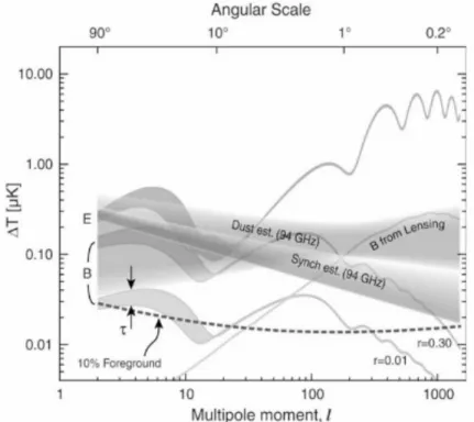
The polarization of the CMB can provide such a handle in the form of B-mode polarization. The spectral and spatial shapes of the foreground emission are significantly different from those of the original B-mode signal.
Galactic science
Cosmological experiments, such as Planck, reflect this in their design, although there are limits to how wide a range of frequencies can be covered by a single telescope.
Design Goals
- Frequency & Bandwidth
- Resolution
- Sensitivity
- Sky Coverage
- Polarization
- Systematic Effects
Cosmological experiments therefore generally try to measure as much of the sky as possible to minimize this problem. To be of greatest benefit, it is therefore necessary for C-BASS to cover as much of the sky as possible.
Experiment Design
- Antennas & Optics
- Receivers
- Scanning
- Pipeline
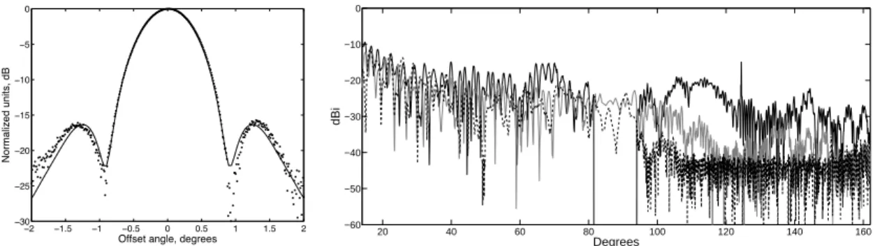
Predictions and measurements of the north main beam and side loop response are shown in Figure 2.5. Coverage of a single hemisphere is guaranteed when scanning at the height of the celestial pole.

Northern Telescope Performance
The reduction of these data demonstrated the proper functioning of the instrument while allowing the first galactic science from C-BASS. The analysis forms part of the scientific content of this PhD degree and is discussed in detail in chapter 7.
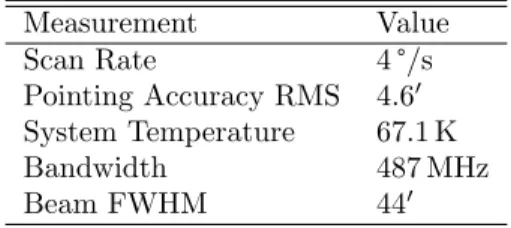
Requirements
The bandwidth of the astronomical signal is relatively small: less than 40 Hz (the actual bandwidth is determined by the scanning speed of the telescope), but is limited to the modulation frequency (and its harmonics). Receiver performance can be monitored via diagnostic signals, a number of which are available for the backend.
Hardware
Timing
Every effort was made to remove this signal from the 1PPS line, but it remained strong enough to confuse accurate measurements of the 1PPS rising edge. 1PPS rising edge detection errors occur on second time scales, but produce timing errors of less than 2 µs and decay quickly.

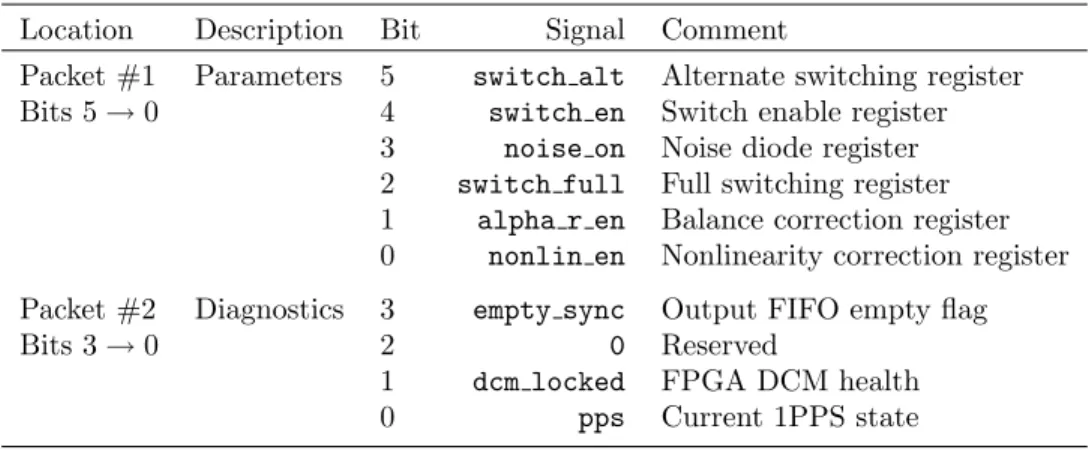
Parameters, Registers, and Diagnostics
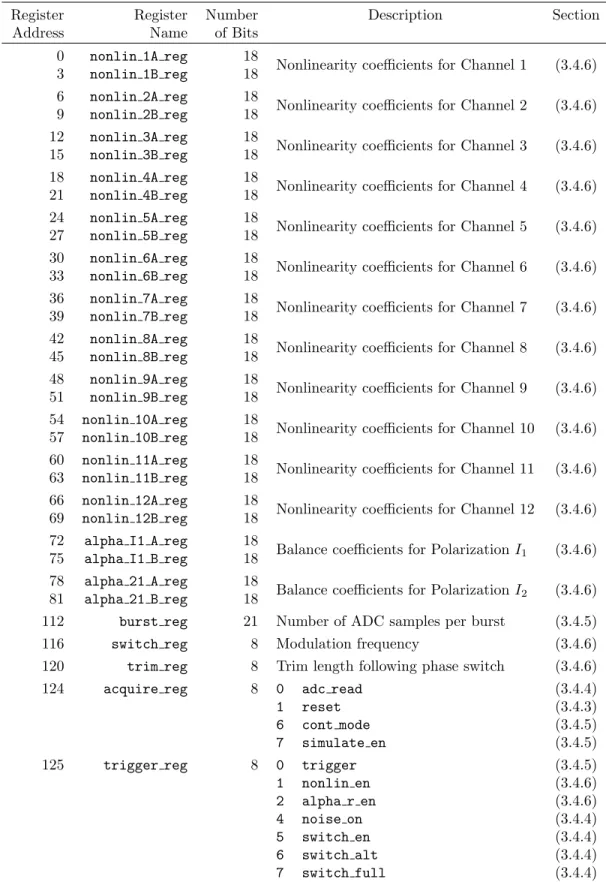
Many diagnostic signals exist outside of the registers and are also available to the user. For burst mode, the parameters (see Table 3.10) are the contents of the trigger reg register as listed in Table 3.6.
Control Signals
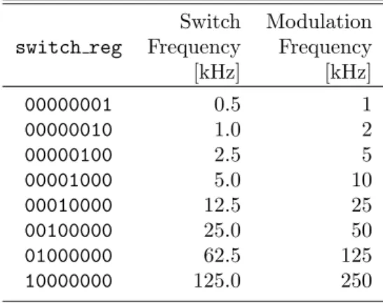
Valid selections can be selected by setting the switch register, as described in Section 3.4.3, and are enforced by the component timing control hc. The rear allows the phase switching to be switched off (via the switch and register), for only one of each pair to be switched (via switch vol), and for the phase switching to be reversed (via switch alt).
Data Acquisition Modes
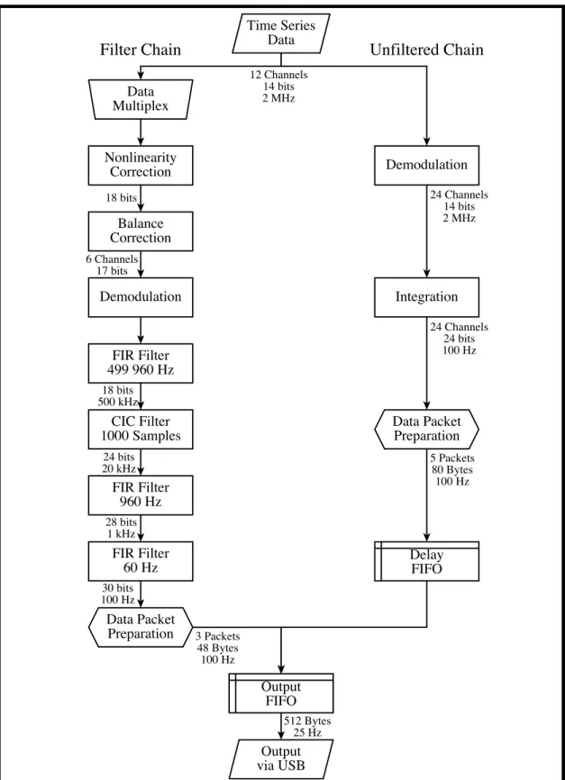
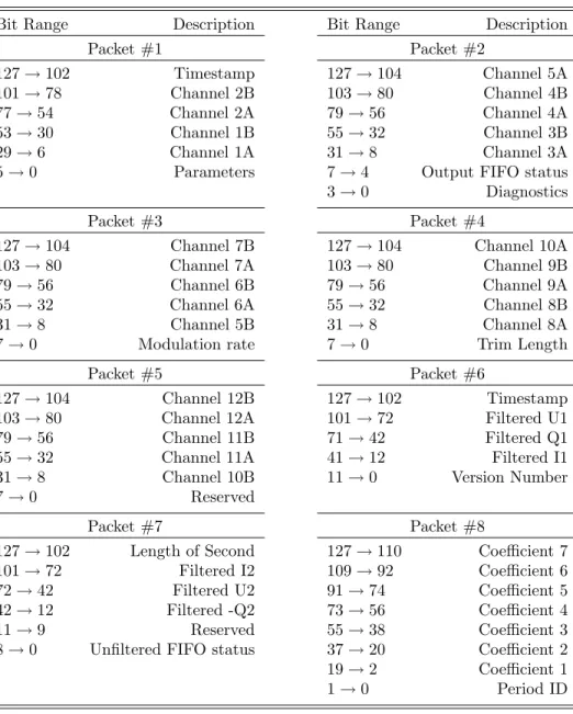
Among these, various control signals and diagnostics are expressed, enabling real-time monitoring of the backend system. The twelve 2 MHz time series are immediately packed into two 128 b packets (described in Table 3.10) and continuously shunted through the secondary FPGA and into the 128 MB SDRAM.
DSP Chain
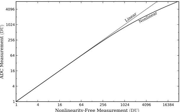
- Multiplicative Corrections
- Demodulation
- Filtering and Integration
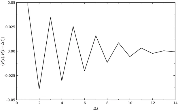
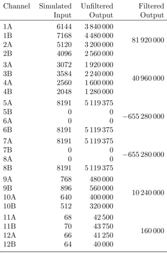
Analytical calculation of the autocorrelation function is precluded by the fractional downsampling in the CIC filter, so it is calculated numerically instead. The redundancy in the paired DSP chains allows for testing the filter performance and fidelity.
USB Microcontroller
FPGA, which was bridged via a dual-clock FIFO, which required two of the FPGA's RAM blocks. After passing through this clock domain interface, the data is sent to the microcontroller via 16b of the FPGA's parallel, 18b output USB input.
Operation in the Field
The end products of the pipeline are calibrated maps of the entire sky in the HEALPix format (G´orski et al. 2005). The pipeline is collaboratively written, with various aspects written and tested by different members of the C-BASS collaboration.
The MATLAB Pipeline
- Initial Flags and Plots
- α Corrections
- Cold Cycle Correction
- r Factor Correction
- RFI Flagging
- Astronomical Calibration
- Summary Plots
- FITS Output
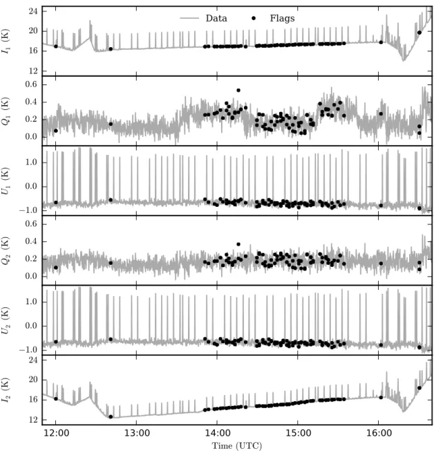
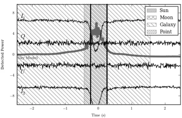
Calibration skydips are referred to as 'current' and 'skydip', while noise diode firings are referred to as 'noise'. The constant altitude during whole sky scans is clearly visible in the altitude graph, with the azimuth scans themselves shown in the azimuth graph. Therefore, unless a factor correction is applied (see section 4.2.4), the total intensity correction becomes degenerate with gain and is therefore not necessary.
The Descart Map Maker
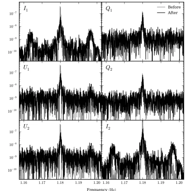
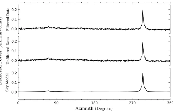
In the I channels, the enhancement by filtering is due to the presence of low-frequency correlated noise. The astronomical signal in the integrated C-BASS time series occurs at frequencies below 40 Hz, with most of the astronomical signal at the lowest frequencies.
Assumptions
The cold cycle frequency is therefore subject to frequency and phase fluctuations present in the electricity grid. Furthermore, due to the uncertainty in the mechanisms involved, amplitude variations in the interfering oscillations must also be taken into account.
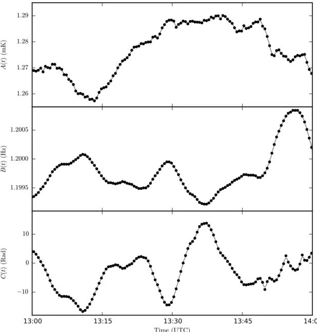
Parameter Measurement
An accurate and precise measurement of the template F(θ) is essential, and this can only be achieved under the assumption that the disturbing signal is consistent over a sufficiently long time scale. If the cold cycle were a perfect 1.2 Hz signal with no phase noise, this value would be a constant zero.
Template Estimation
A 1.1 Hz high-pass filter is applied to each channel, removing much of the astronomical signal and 1/f noise. As mentioned above, this is done for all 20 unique outputs of the different modes of the correction.
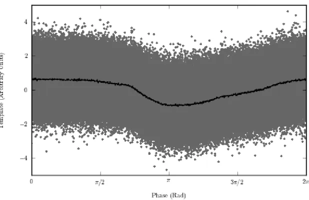
Template Fitting
Each time the C-BASS observer updates the template scores, the observer must judge where there are qualitative changes in the behavior of the scores. Finally, the templates are repeated for three periods and low-pass filtered with a cutoff of 60 Hz.
Discussion
This shows the need for both this algorithm and for maintaining good health of the recipient. Statistical notation is emphasized, as it constitutes a significant part of the work of this thesis.
Analog Filtering
Spatial Flagging
Statistical Flagging
Assumptions
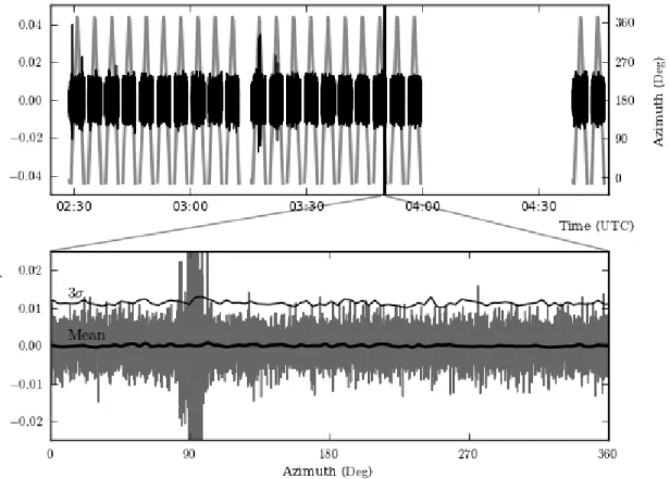
Rapidly varying RFI will excite time series frequencies inaccessible to the C-BASS antenna and scanning strategy. The astronomical structure will only be able to contribute to time series frequencies below the ratio of scan rate to beam size.
Flagging Procedure
These four σX,T(t) time series are then compared in a manner that preferentially highlights RFI over non-RFI data. Once calculated, the averages of the total intensity time series are taken as σI,0.25(t) and σI,0.5(t), and the maxima of the linear polarization series are taken to be σP,0.25(t ) and σP,0.5. (T).
Parameter Tuning
Statistical reporting is also produced for parameter groups in which the parameters have changed by 10% from the suggested values. The statistical flags from the suggested parameter sets are then consolidated with the folded candidates to produce a master list of RFI candidates.
Discussion
The anomalous microwave emission (AME) was first discovered in observations near the North Celestial Pole (NCP) by Leitch et al. In addition, Draine & Lazarian (1998a) argued that the free-free hypothesis of Leitch et al. 1997) was unlikely due to the energy injection rate required to keep the gas so hot.
C-BASS Data
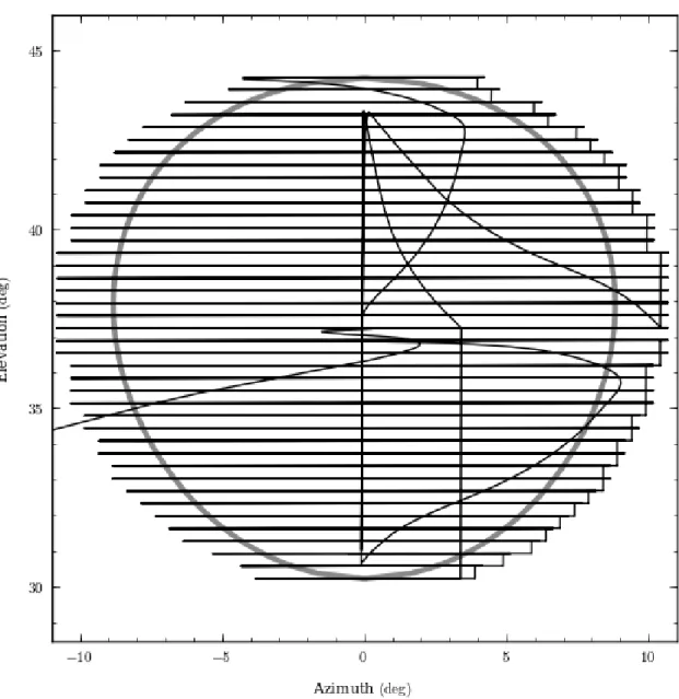
The antenna target track shows the scans over the field and the sky dips. Compression and rarefaction of the scans at 12 o'clock and 0 o'clock respectively are due to the Earth's rotation during the observation.
C-BASS Analysis
This is likely due to an error in the assumed flux density of the end source. A further noise test is performed by filtering the kernel-reduced time series.
Multiwavelength Comparison
The map pointing and calibration test was performed by fitting a Gaussian function to the 3C61.1 point source. Although a detailed cross-correlation analysis is beyond the scope of this work, the new C-BASS map is briefly compared with existing maps to demonstrate the utility of C-BASS data.
Discussion
Anomalous microwave emission has now been observed by many authors in a variety of galactic and extragalactic environments (Finkbeiner et al. Most recently, Hoang et al. 2013) used the polarization feature of 2175 ˚A, as observed for two stars, to argue that the polarization of spin dust should peak at 3% at 5 GHz, and decline rapidly above 20 GHz.

Overview
As this approach uses the Fokker-Planck equation instead of the Langevin equation, it is not possible to reproduce the transient spin-up effects of HDL10. The strategy adopted in this work is to make a number of reasonable simplifications aimed at approximating equation 8.4 as a log-normal distribution function.
Dust Grains
- Size
- Shape
- Temperature
- Charge
- Dipole Moment
In section 8.5.1 the effects of geometry and irregular rotation are parameterized as part of the full derivation. The intrinsic, electric dipole moments of the grains are observationally poorly constrained, and attempts to derive them theoretically are subject to uncertainty in the specific chemical compositions of the grains.
Distribution Function
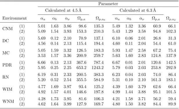
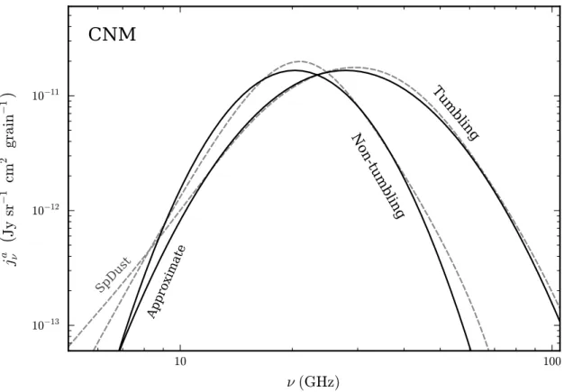
In quantifying these assumptions, this equation serves as the definition of the power law indices and the peak rotation frequency Ωp,a0 for grains of sizea0. Curves calculated from SpDust are compared with the results of the power law approach (extrapolated from 4.5 ˚A grains).
Emissivity
Grain Tumbling
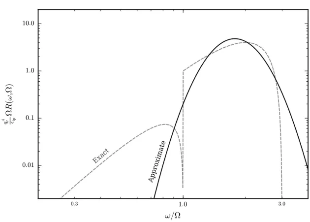
This shape obviously allows for the various permutations of grain geometry and rotational dynamics, with the emission spectrum itself contained in the R function. In the case of tumbling, there is emission due to the in-plane and out-of-plane electric dipole moments.
Grain Emissivity
The results can be applied to non-tumbling cases by setting σr= 0 and R0 equal to the coefficients in Equations and 8.25. This is plotted in Figure 8.5 for disk-like grains in both the tumbling and non-tumbling cases.
Total Emissivity
The components of this function are shown in Figure 8.6, in which the power-law and log-normal components are shown in turn, as well as the complementary error function. The model is demonstrated through comparison with Perseus Molecular Cloud data of the Planck Collaboration (2011) in Figure 8.10.
Discussion
This work bypasses the lengthy numerical calculations of previous models while encouraging an intuitive picture of the radiation. Each step of the derivation was tested against numerical calculations to demonstrate accuracy.