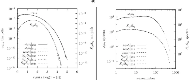
Note that the volume pdfs use a sign transformation of the form (x) log (1 +|x|) in abscissa coordinates and that the curves for the fields ωiωi and SijSij use two different vertical axes (both in the pdf and in the spectra) , shifted a decade for a clear view (non-crossing curves). Each point of that function (right) represents the area (two-dimensional Hausdorff measure) of the associated part.
Previous identification criteria
Regions of points can then be formed that share a common identity based on the local criterion used, but often this local analysis is the end of the identification process. While local methods are often based on a priori physical knowledge of the particular geometry to be developed, nonlocal methods generally draw physical conclusions a posteriori based on geometric features obtained from the developed structures.
Non-local, multi-scale, and clustering features
Choice of applications: passive scalar, enstrophy, and dissipation fields
In the presence of a uniform mean scalar gradient of magnitude µc in the x1 direction – which will be preserved by the flow (see Corrsin, 1952) – the passive scalar can be broken down into its mean component, µcx1, and the passive scalar fluctuation , c0( x, t). They are obtained, up to and including the scale factors, from the double contraction of the tensor fields with rotational and elongation rates.
Grid resolution effects
Structure interaction
Outline
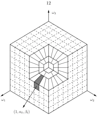
The starting point of this methodology is a three-dimensional scalar field obtained from a turbulence database.
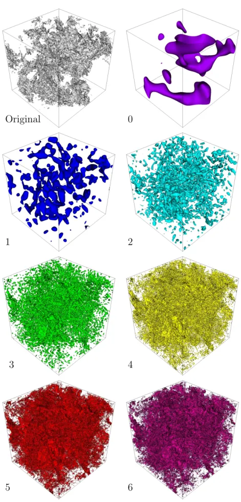
Extraction of structures
The curvelet transform
Curves, the basic functions of a curve transform, are localized in scale (frequency/Fourier space), position (physical space), and orientation (unlike wavelets). See Appendix B for a physical interpretation of the formed structures after this multiscale decomposition and isocontouring procedure.
Periodic reconnection
After this multi-scale analysis, a second step is used in the extraction process to generate structures of interest associated with each relevant range of scales. Currently, these structures of interest are defined as individual disconnected surfaces obtained by isocontouring each filtered scalar field at specific contour values (for example, the mean of that filtered scalar field plus a multiple of its standard deviation).
Characterization of structures
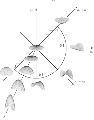
Shape index and curvedness
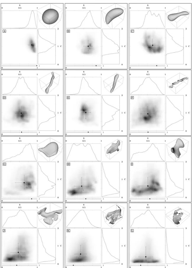
Thus, higher curvature values correspond to a smaller radius of curvature (and consequently a more locally curved surface at P). The absolute value of the shape index S ≡ |Υ| represents the local shape of the surface at point P, where 0≤S ≤1.
Joint probability density function (jpdf)
Another dimensionless global parameter useful in characterizing the geometry of molded closed structures is. It represents the stretching of the structure; the smaller its value, the more stretched the structure is.
Signature of a structure
The value of the stretch parameter, λ, is represented below the jpdf with a black bar (on a scale from 0 to 1). The only modification is the way in which the normal vector is calculated on each face of the discretized surface, following the method proposed by Chen & Wu (2004).
Classification of structures
Clustering algorithm
The element of the distance matrix measures the dissimilarity between two elements of e-endejofE, based on their signatures. The K-means clustering algorithm mentioned above is one of the simplest partitioned clustering techniques available.
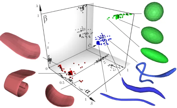
Feature and visualization spaces
The feature center ( ˆS, ˆC) takes into account the asymmetry of the jpdf, and corrects the mean center ( ¯S,C) so that the feature center is closer to the region of ¯ higher density of the jpdf. In general, the higher dimensional nature of the feature space prevents its use as a visualization space, but the utilization of glyphs, scaling, and coloring allows more than just three dimensions to be represented in the visualization space.
Optimality score: silhouette coefficient
It is a confidence indicator of an element's membership in the set it is assigned to. Each sphere in that space represents a virtual array structure (some examples are projected onto planar sides).
Multi-scale diagnostics
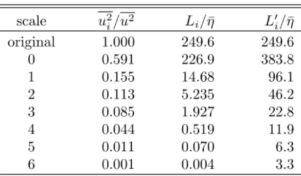
From this observation and from Figure 4.3(a) we note that those pdfs associated with the degrees corresponding to the inertial ranges (1, 2 and 3) are very similar, almost collapsing in that. This allows us to define the squared integral characteristic velocities,u2i and integral length scales,Li,L0i, for each filtered scale,i, in the same terms in which they were defined for the original velocity field.
Geometry of passive scalar iso-surfaces
The thickness of these bars is also scaled by the value of the silhouette coefficient. Note how the glyphs in Figure 4.8, scaled by the renormalized silhouette coefficient of the associated structures, are smaller in the overlapping regions (compare, for example, Figure 4.5 (top), where the point density is much higher continuous throughout the distribution, since the scaling factor in that case was the area of the structure, not its silhouette coefficient).
Discussion and physical interpretation
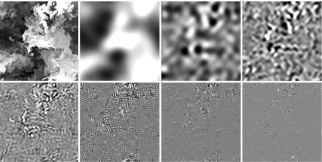
These features are visible on large scales (plateau regions) as well as on small scales (cliff fronts) where there are steep changes in passive scalar values (see Figure 4.2). As of now, ScandRe is not aware of any previous reports of tubelike and tubular (moderately stretched) structures in the intermediate scales of the passive scalar fluctuation field.
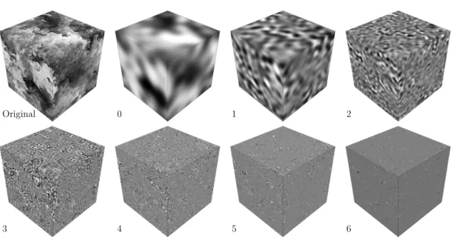
Multi-scale decomposition
Note that the volume pdfs use a transformation of the form sign(x) log(1 +|x|) in the abscissa coordinate, and that curves for ωiωiandSijSij fields use two different vertical axes (both in the pdfs and the spectra), shifted one decade for a clear view (non-crossing curves). Volume pdfs (physical domain) and spectra (Fourier domain) of the original and component fields after the multiscale decomposition are shown in Figure 5.3, for ωiωi(top) and SijSij(bottom) fields in the 10243 case.
Characterization and classification of individual structures
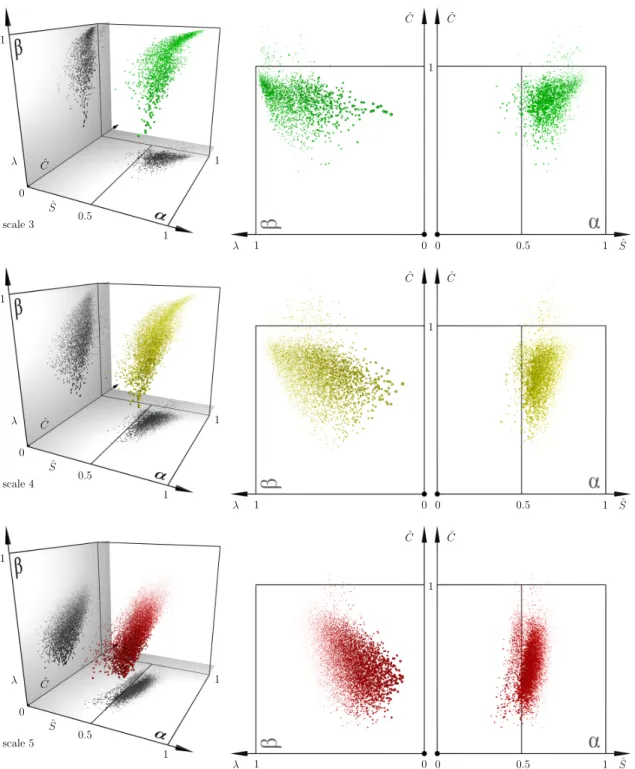
On the other hand, the SijSij structures are less concentrated in the tube-like region (see Figure 5.8 and compare the scale numbers 3 and 4 of SijSij in Figure 5.10 with those of ωiωi in Figure 5.12), while they show, at all scales of intermediate, many more structures with smaller ˆC values, characteristic of sheet-like geometries. The transition to sheet-like structures begins earlier, at scale number 3, for SijSij than forωiωi, and is completed by scale number 5.
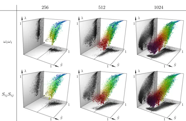
Effect of grid resolution in the geometry of structures
Compared to the homologous scale number for the higher grid resolutions, it can be seen that the strong sheet-like character of the structures is not well captured in 2563. A possible explanation is that at that resolution sheet-like structures are more fragmented into smaller structures (part of the original ).
Clustering results for the 1024 3 case
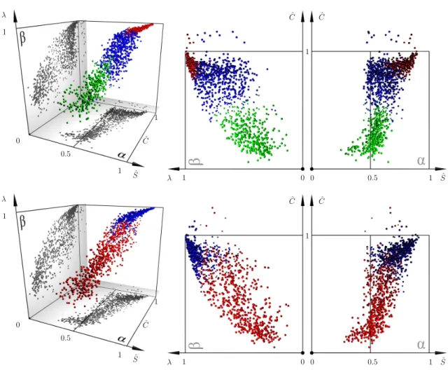
Glyphs are scaled by the normalized value of the silhouette coefficient, which indicates the degree to which this element belongs to the assigned group. The optimal number of clusters (square point) of 3 and 2 was automatically determined for ωiωi and SijSij, respectively.
Discussion
The aim is to provide a qualitative and quantitative assessment of the geometric aspects of those local identification criteria. Note that the volume PDFs use a transformation of the form sign(x) log(1 +|x|) in the abscissa coordinate, and that curves for Q and [Aij]+ fields use two different vertical axes ( both in the PDFs and in the spectra), shifted by a decade for a clear picture (non-intersecting curves).
Application of non-local methodology
The visualization spaces in Figure 6.4 contain glyphs corresponding to the geometric characterization of the individual structures shown in Figure 6.3, with the same color scheme (blue used for Qstructures and red for [Aij]+structures). This could be anticipated by looking at the organization of glyphs in the visualization space in Figure 6.5, compared to Figure 5.13.
![Figure 6.2: Plane cuts of Q (left) and [A ij ] + (right) fields normal one of the principal directions of the cubic domain, at half its side length](https://thumb-ap.123doks.com/thumbv2/123dok/11088128.0/91.918.179.800.115.421/figure-plane-fields-normal-principal-directions-domain-length.webp)
Methodology
Processing individual structures
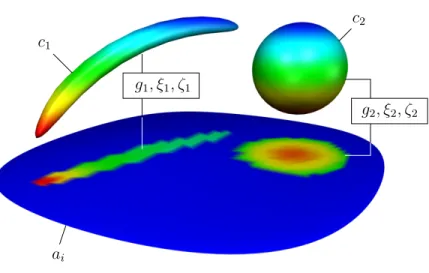
Those points of ai labeled during the computation of the minimum distance maps (with closeness values greater than zero) will also store the {gj, ξj, ζj} values of the corresponding cj in the conditional string map. A scheme of calculating the steps of the conditional string map based on the minimum forcj distance maps is shown in Figure 7.2.
Transition from individual structures to results for the set A
Computational remarks
However, we note that this imposes the additional constraint that the discretized surfaces sai and cj must have equivalent grid resolution for accurate calculation of the distance maps underlying this algorithm. In our implementation, this is ensured as a result of the isocontouring algorithm used and the fact that no subsampling was performed on the grid for any scale, even when multiscale techniques were used, and no decimation operation was performed. which is then applied over the discretized structures.
Proximity and area coverage of surrounding structures through jpdf+i
Unsaturated regions indicate less areal coverage, and colors closer to the blue hue indicate lower proximity values (and thus, more distant structures). Deep blue regions, for example, would indicate that the structures of B with those (ˆS,C) values appear far away, but cover a large part of the surfaceˆ of the structures of A.
![Figure 7.3: Components of the jpdf+i in terms of ( ˆ S, C), plus intensity component based on proxim- ˆ ity, of structures of X (Q)∪ X ([A ij ] + ) surrounding structures of X (Q): area-coverage pdf component (top left) using greyscale; intensity component](https://thumb-ap.123doks.com/thumbv2/123dok/11088128.0/103.918.171.796.94.685/components-intensity-component-structures-surrounding-structures-component-greyscale.webp)
Proximity split by groups through cumulative marginal pdfs
Examples of this interaction obtained from the studied database are shown in Figure 7.5, examples (a), (b) and (c). For some examples of this configuration, see examples (d), (e) and the plates surrounding the pipes in example (f) in Figure 7.5.
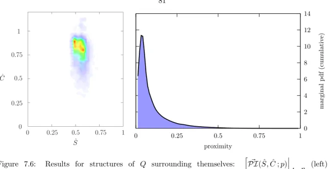
Structures of Q surrounding themselves
The contribution of [Aij]+ (red area) to the marginal pdf in Figure 7.4 shows four regions of interest: first, the region close to unity (p≈ 1), which corresponds to [Aij]+ structures very close to those of Q , are likely to overlap / intersect with each other. Third, the region with proximity values between 0.25 and 0.5 with low marginal pdf values indicates that surrounding structures are rarely found at those distances.
In the first case, i.e. for the set B containing the structures ωiωi, two saturated regions are present on the surface (meaning high surface coverage), which correspond to the tubular (closer to ( ˆS,C)ˆ ≈ ( 1/2,1) and sheet (small values of ˆC) structures. In the second case, SijSij structures at each of the analyzed scales (3-6) have a more balanced contribution to the marginal pdf; scale number 3 shows a slightly higher concentration of closer structures (p > 0.6) and a smaller proportion of distant structures (p≈0.1) compared to structures on scale 4–6.
Discussion
Secondly, the study of the structures derived for the different scales shows a transition of their geometry from predominantly the blob-like and tube-like type in the inertial range of the scales to plate-like structures in the dissipation range. This suggests the need to solve sub-Kolmogorov scales for a proper geometric study of the smallest structures of intermittent fields in turbulence, as previously reported in the literature (see Shumacher & Sreenivasan, 2005; Horiuti & Fujisawa, 2008).
Assessment of non-local methodology complementing existing local identification criteria 87
A small amount of structures in both fields present a geometry that does not correspond to the expected shape. When ωiωi on the same intermediate scale is studied in relation to the structures of SijSij.
Computational remarks
Two groups of surrounding geometries are dominant: plate-like structures are closer; tubular structures are further away, but they cover a large part of the surface area of the structures that surround them, thus indicating that the nearby plate-like structures do not obscure them. Plate-like geometries are again the closest, and appear to revolve around the tubes of ωiωi, more effectively obscuring other more distant geometries.
Future work
Considering the explanation of the character of δ[Mξ=], the function f(ξ) can be interpreted as the average value of the variation with ξ of µ2/µ1 in the set Mξ= (expressed as d[µ2/µ1|Mξ =/dξ) . This formula relates the geometry of the surface (given by the integration of the Gaussian curvature, a property of differential geometry) to its topology (given by the Euler characteristic).