We present a robust 2D shape reconstruction and simplification algorithm that takes as input a set of points loaded with errors, noise and deviations. We introduce an approach based on optimal transport, where a set of input points, treated as a sum of Dirac measures, is approximated by a simplicial complex, treated as a sum of unitary measures on 0- and 1-simplices. A fine-to-coarse scheme is devised to construct the resulting simplicial complex by greedily decimation of the Delaunay triangulation of the input point set.
While some authors (especially in Computational Geometry) have limited the reconstruction problem to finding a connection of all input points, the presence of noise and the large size of most data sets requires that the final reconstructed form be more concise than input.
Previous Work
Reconstruction
Simplification
Contributions
Outline
Applications
In computer graphics, optimal transport theory has recently been applied to geometry processing tasks such as shape inference and registration. 8], for example, exploited optimal transport theory to design approximations of unsigned distance functions that are robust to noise and outliers. In computer vision, optimal transport has also been used as a means of comparing [37], transferring [11] and quantizing colors in images [6].
35] used optimal transport to derive tight bounds on the accuracy of discrete differential operators and then formulated a family of functional elements for mesh optimization.
Formulation
Benefits
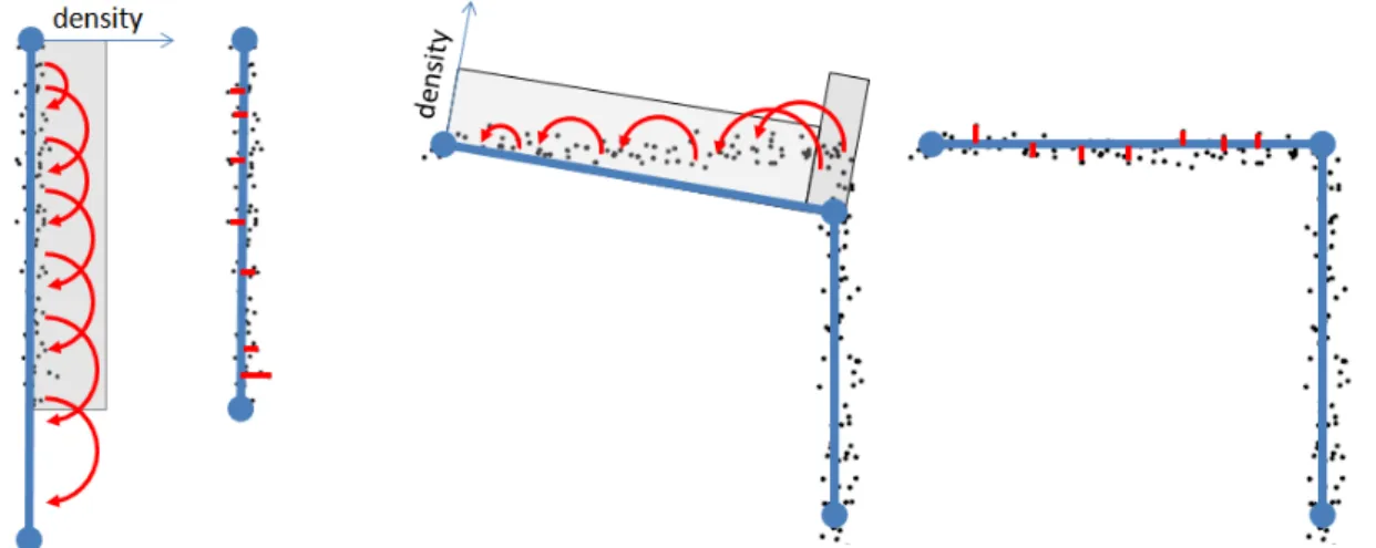
The main advantage of the idea of optimal transport distance in the context of reconstruction and simplification is its robustness against noise and outliers [8]. Second, the optimal transport cost measures the local lack of uniform sampling of the point set along the reconstructed edges; minimizing such a metric favors edges that cover uniformly dense regions while preserving boundaries and sharp features (Fig 2.1). Left: An edge that extends past (or short of) the point set will acquire a large tangential component, which enforces the preservation of boundaries.
Right: When an edge does not fit an acute corner, the transport cost has both a large tangential component (due to the non-uniform sampling along the edge) and a large normal error.
Transport Plan & Cost from Points to Simplices
Points to Vertex
Points to Edge
The tangential plan is a little more complicated to derive, but its costs can also be done in closed form. Each point qi is then spread tangentially across the i-th bin, creating a uniform measure across e, defining the local optimal transport from Se to e (see inset). Now consider a point pi of mass mi projecting onto qi on edgee; set a 1D coordinate axis along the edge with the origin at the center of the ith bin, and name the coordinate of qi in this coordinate axis.
The tangential cost ti e pi is then calculated as the cumulative distribution resulting from the 1st-order moment of all points in the ith bin with respect to the projection, giving: We can now sum the costs for each point pi in Se to obtain the tangentialT component of the optimal transportation cost for an entire edge:. 2.5) is correct; it is thus stable in processing, in the sense that we get the same cost if we divide each mass point into several points that summarize the volume and transport them in smaller bins whose lengths are a function of the new masses.
The total cost W2 of transporting S to T through the transport plane π is thus conveniently written by summing the contributions of each edge and vertex of T:.
Point-to-Simplex Assignment
We then go over each edge and consider the two following assignments: either (i) keep Se assigned, or (ii) instead assign each point of Se to its nearest endpoint or we choose, from these two possibilities, the local assignment that results in the smallest total cost. Once this simple test is performed for each edge, the verticesv and edgeseofT all have their assigned points (SeandSv, respectively) from S, and the optimal transport plan (and cost) for this assignment is therefore fully determined as derived in Sect. Note that this assignment provides a natural characterization of the edges of T: an edge is called aghost edge when Se=∅, i.e. no import points are transported on it; conversely, it is called solid edge if it receives a non-zero amount of mass from the point collection.
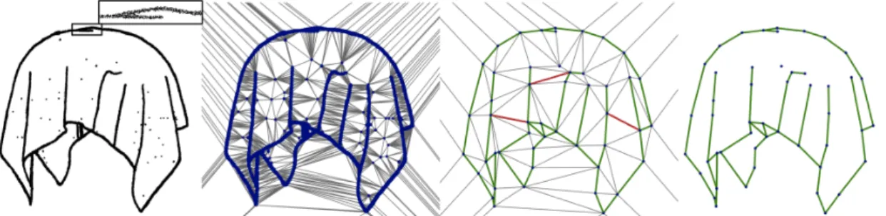
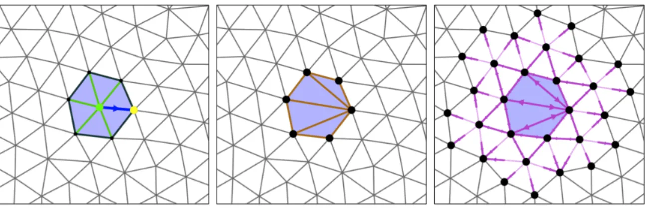
Ghost edges are not actually part of the reconstruction and are only useful to define the current simplicial tiling of the domain (see Figure 3.1, center right). Using the point-to-simplex mapping and associated induced transport plan described in the previous chapter, we now devise an algorithm to produce a coarse reconstruction based on the input point set. From left to right: input point set; Delaunay triangulation of input; after simplification, with ghost edges in gray, relevant solid edges in green, discarded solid edges in red; final reconstruction.
The algorithm proceeds in a fine-to-coarse fashion by greedy simplification of a Delaunay triangulation initialized from the input points. Simplification is performed by means of a series of half-edge collapse operations, so ordered to minimize the increase of the total transport cost between the input point set and the triangulation. Vertices are also locally optimized after each edge collapse to further optimize the local allocation.
Initialization
Simplification
Systematically Collapsing Edges
A half edge is said to be collapsible if its collapse causes neither overlaps nor folds in the triangulation. To preserve the triangulation embedding, we need to focus only on foldable edges during simplification. Although simple and commonly used, these validity conditions invalidate approximately 30% of candidate collapse operators during the entire course of a simplification.
This can seriously affect the performance of our greedy approach to optimal transportation, as it relies on targeting the edge with the least cost first. We denote by Pxi the (counterclockwise oriented) polygon formed by the en-ring of xi, and by Kxi its core. The idea of the reversal procedure is to extend Kxi in the direction of (xi, xj) until it includes xj.
We then sort the blocking edges into a priority queue in descending order of distance D and select the top edge to be removed from Pxi. Note that, since (a, b) has the largest distance D within Pxi, either (a, xi) or (b, xi) can rotate, otherwise (a, b) would not be at the top of the queue. Between these two choices, we choose the edge with the smallest When flipped, since it takes longer Kxi.
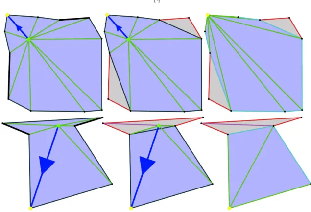
By repeating the flipping of the edges, we iteratively move Kxi towards xj and this process will definitely end when the changed Pxi has no more blocking edges (Figure 3.5). It should be noted that xi may not be inside the final Pxi (Figure 3.5, bottom); however, since the flipping process is always associated with the collapse of half the edges, xi is subsequently deleted by the collapse, leaving the mesh always valid.
Vertex Relocation
To solve this problem and ensure that the greedy decimation is systematically processed in increasing order of cost, we adapt the collapse operator via a local edge-flip procedure that makes each edge collapsible, as we now consider. We also call an edge reversible if its endpoints and the two opposite vertices form a convex quadrilateral. Left: Collapsing the edge (in blue) causes wraps due to blocking edges (in black).
Recall that the square of the normal part of the W2 cost associated with a vertex of T can be written as. In practice, we move the vertex v tov∗ only if the resulting triangulationTk+1 is still an embedding (i.e. v∗ is inside the core of the uniring ofv). Once this relocation is achieved, we proceed as we did for edge collapses: we collect the input points affected by this shift, assign them to their nearest edge, and determine the new transport planπk+1.
Edge Filtering
Implementation details
- Initialization
- Multiple-Choice Priority Queue
- Postponing Vertex Relocation
- Reconstruction Tolerance
For large data sets, a significant speedup can be achieved by using only a random subset of the input points for T0. The reconstruction of large data sets requires the simulation of thousands of collapse operations, and therefore our algorithm initially spends a significant amount of time performing frequent updates of the dynamic priority queue. Vertex moving is only effective when a sufficient number of input points are assigned to each edge of the triangulation.
Obviously, this number is very small at the beginning of the algorithm and increases as the triangulation becomes coarser. For this reason, we turn off the vertex shift step during most of the simplification process, and only enable it for the last 100 decimations. It takes as input point sets, possibly with mass properties, and a desired vertex count of the final reconstruction.
On closed and noise-free curves, our approach performs comparably to state-of-the-art reconstruction and simplification methods applied in sequence. Our reconstruction is perfect for a noise-free input (left); as noise is added (middle, 2% and 2.5% of the bounding box), the output degrades gracefully, still capturing most of the sharp corners; even after adding 4K or 4.5K outliers and 2% noise (right), the reconstruction remains of high quality, although artifacts start to appear in this regime. The original assignment for T0 implies a vertex discretization of the data sets since all edges are initially classified as ghost edges; then these vertices are regrouped into 1-simplices, which first consolidates the reconstruction of highly sampled regions.
Finally, as the triangulation is simplified, we get a rough scale approximation of the input data. We compare our approach (right) with two curve-simplification algorithms: QEM [20] (left-center) and Douglas-Peucker [22] (center-right). The lines of the derived shape near the star center are visually indistinguishable (see close-up).
Reconstructing the curve: Connecting the dots with good reason. Proceedings of the 15th Annual ACM Symposium on Computational Geometry.


![Figure 4.2: Bird. Top: For a closed and noise-free point set, combinatorial methods such as crust [21] finds a connectivity for all input points, while we obtain a simplified reconstruction](https://thumb-ap.123doks.com/thumbv2/123dok/11464901.0/24.892.194.779.439.734/figure-closed-combinatorial-methods-connectivity-points-simplified-reconstruction.webp)
