In this revised and improved second edition of Optimization Concepts and Applications in Engineering, the already robust pedagogy is enhanced with more detailed explanations and a greater number of solved examples and end-of-chapter problems. This book can be used in courses at the graduate or senior undergraduate level and as a learning resource for practicing engineers.
Introduction
A CD-ROM is available containing computer programs that parallel the discussion in the text. Software development has also helped explain optimization processes in written text with greater insight.
Historical Sketch
The most notable of these are genetic algorithms [Holland 1975, Goldberg 1989], simulated annealing algorithms derived from Metropolis [1953], and differential evolution methods [Price and Storn, http://www.icsi.berkeley.edu /∼storn/code .html]. Also available are GAMS modeling packages (http://gams.nist. gov/) and CPLEX software (http://www.ilog.com/).
The Nonlinear Programming Problem
Structural optimization and simulation-based software packages available for purchase by companies include ALTAIR (http://www.altair.com/), GENESIS (http://www.vrand.com/), iSIGHT (http: //www. .engineous.com/), modeFRONTIER (http://www.esteco.com/) and FE-Design (http://www.fe-design.de/en/home.html). Mixed Integer Programming (MIP): an IP where some variables are required to be integers, others are continuous.
Optimization Problem Modeling
Let (wi,hi),i=1, 2, 3, denote the width and height of the cell, and (xi,yi) denote the coordinates of the lower left corner of the cell. Power produced by each FA depends on the enrichment of the fissile material it contains and its location in the core.
Graphical Solution of One- and Two-Variable Problems
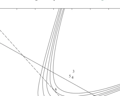
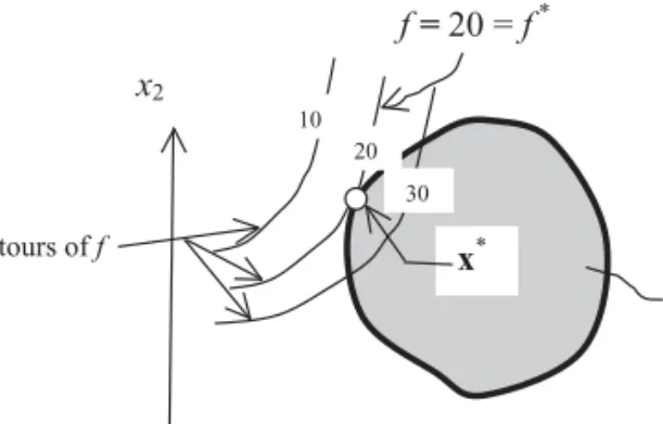
Draw (i) a 3D plot of this function and. ii) a contour plot of the function in the variable space orx1–x2space. Then the feasible side of the curve can be easily identified by checking wheregi (x)<0.
Existence of a Minimum and a Maximum: Weierstrass Theorem A central theorem concerns the existence of a solution to our problem in (1.1) or
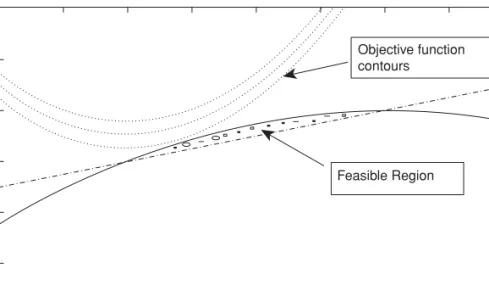
While it is true that a solution may exist even if the conditions are not met, this is highly unlikely in practical situations due to the simplicity of the conditions. A look at the feasible region shows that it is unbounded, which violates the simple conditions in the Wierstraas theorem (Fig. E1.14b).
Quadratic Forms and Positive Definite Matrices
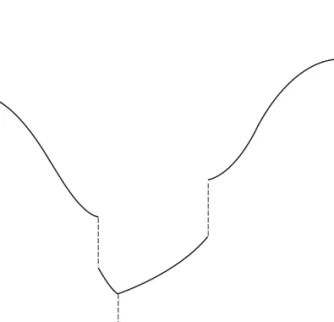
While the graph of the function gversusxi is “disconnected,” the function is continuous at every point in its domain because of the way it is defined.
Gradient Vector, Hessian Matrix, and Their Numerical Evaluation Using Divided Differences
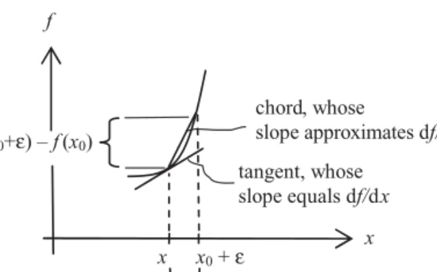
Newton's forward difference formula is often used to obtain an approximate expression for ∇f (and also for ∇2f) at a given point. Evaluate the derivative of the second or highest eigenvalue with respect to tox, dλdx2, at the point x0=0.
Taylor’s Theorem, Linear, and Quadratic Approximations
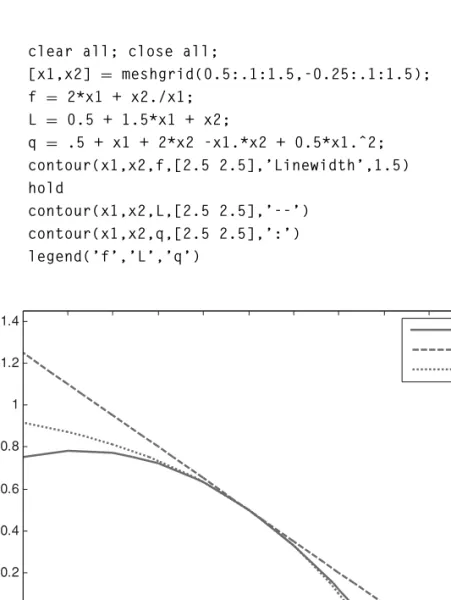
Construct linear and quadratic approximations to the original function fat x0 and draw contours of these functions passing through x0.
Miscellaneous Topics
Roos, C., Terlaky, T., en Vial, J.P., Theory and Algorithms for Linear Optimization: An Interior Point Approach, Wiley, New York, 1997. Schmit, L.A., Structural design by systematic sinthesis, Proceedings of the 2nd Conference on Elektroniese berekening, ASCE, New York, pp.
Introduction
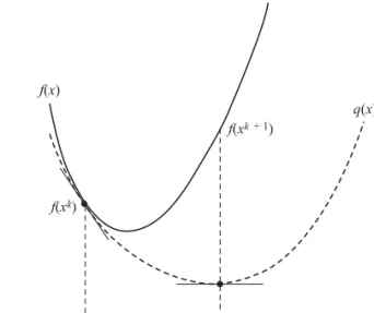
Theory Related to Single Variable (Univariate) Minimization We present the minimization ideas by considering a simple example. The first step
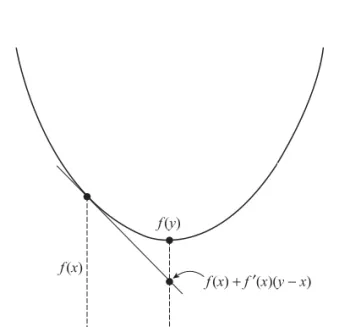
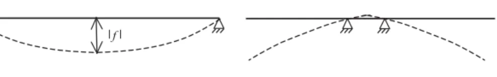
A function f(x) is called aconvex function defined on the convex set S if for each pair of pointsx1andx2inS and 0≤α≤1, the following condition is satisfied f(αx1+(1−α)x2)≤αf(x1)+( 1 −α)f(x2) (2.7) Geometrically, this means that the graph of the function between the two points lies below the line segment connecting the two points on the graph as shown in fig. In this case, one must be careful. as convexity aspects of the original function are completely changed.
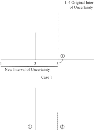
Unimodality and Bracketing the Minimum
Fibonacci Method
A small δ(δIn) can be introduced in the final step to set the uncertainty interval. Without loss of generality, assume that the uncertainty interval is the left interval, that is, [0.5/8].
Golden Section Method
The interval reduction strategy in the golden ratio algorithm follows the steps used in the Fibonacci algorithm. The basic golden ratio algorithm is similar to the Fibonacci algorithm, except that α is replaced at step 4 by the golden ratioτ (= √5−12.
Polynomial-Based Methods
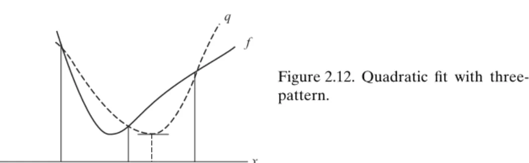
The quadratic fit is accepted if the minimum point is likely to fall within the interval and is well conditioned, otherwise the new point is introduced using golden ratio. Start with three-point patterna,b, andxmeta,b, forming the interval and smallest value of the function atx.
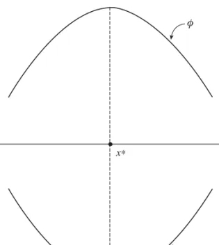
Shubert–Piyavskii Method for Optimization of Non-unimodal Functions The techniques presented in the preceding text, namely, Fibonacci, Golden Section,
Using MATLAB
Zero of a Function
The base of the pyramid is a square with the corners touching the base of the hemisphere. Hint: The wetted perimeter is the length of the underside and the sum of the lengths of the two slanted sides.).
Introduction
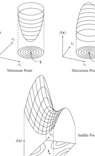
Necessary and Sufficient Conditions for Optimality
The geometric significance of (3.5) is related to the concept of convexity, which is discussed next. No solution exists (in an unbounded domain), which implies that there is no local minimum for this function.
Convexity
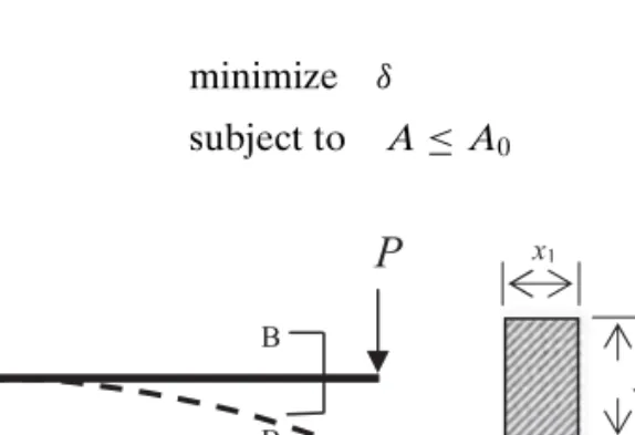
The actual choice of the direction vector and the step size differs among the various numerical methods, which will be discussed subsequently. The design variables are assumed to be the width and height of the rectangular cross-section.
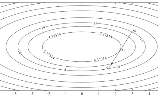
The Steepest Descent Method
The steepest descent direction atx0 is the negative of the gradient vector that gives (−4, −4)T. The term 'global convergent' is used, but this should not be confused with finding the global minimum; the method only finds a local minimum. contains an excellent discussion of the global convergence requirements for unconstrained minimization algorithms.
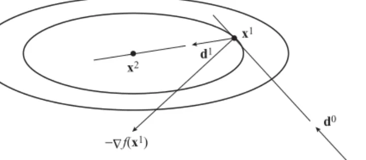
The Conjugate Gradient Method
The Hessian of the new function has the best possible conditioning with contours corresponding to circles. However, numerical line search must be performed to find α instead of the closed form formula in (3.31).
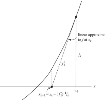
Newton’s Method
To overcome the two pitfalls of Newton's method as discussed in the preceding text, two modifications can be made. An example of this occurs in nonlinear least squares problems as discussed below.
Quasi-Newton Methods
In the matrices on the right-hand side of the previous equation, the superscript has been omitted. Note the following changes to make when switching from one problem to another in the code:.
Approximate Line Search
Since even very small values of α can also satisfy (3.49), a second requirement to ensure convergence is to ensure that α is not too close to zero. An example is given below to illustrate the two criteria for determining [αL,αU].
Using MATLAB
Find the largest rectangular area available within the annular footprint of the robot's workspace (Figure P3.14). i) Construct linear and quadratic approximations of the function f =x1x22 at the point x0=(1, 2)T. Obtain the spring forces by minimizing the potential energy in the system given by z=5. 2kiδi2−Pδ, where δi=vertical deflection of the ith spring and δ=vertical deflection under load.
Introduction
Linear Programming Problem
We note that the number of constraints ism=+r+q,cj and ai j are constant coefficients, biare fixed real constants, which are adjusted to be nonnegative; xyears the unknown variables to be determined.
Problem Illustrating Modeling, Solution, Solution Interpretation, and Lagrange Multipliers
Labor costs less than $10/hour will increase the objective value, labor costs more than $10/hour. 10/hour will decrease the objective value, and labor costs of exactly $10 will keep the objective function value the same.
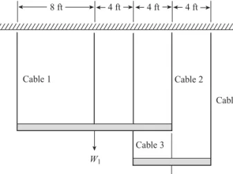
Problem Modeling
Letx1,x2,x3,x4,x5 be the number of kg of each of the available alloys melted and mixed to form the required quantity of the required alloy. Assuming fertilizer costs are the same for each product, determine the optimal crop combination.
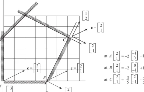
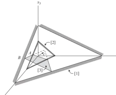
Geometric Concepts: Hyperplanes, Halfspaces, Polytopes, Extreme Points
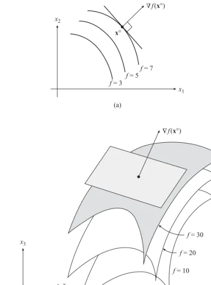
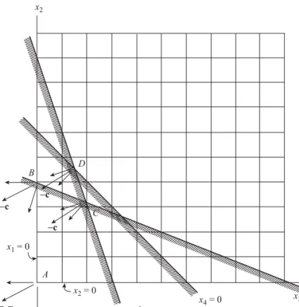
Similarly, the gradients of the constraints are [2,−1]T,[1,2]T,[−1,1]T, respectively, and [−1,0]T,[0,−1]T for limits remember from the previous chapters that the gradient is normal or perpendicular to the limit and points in the direction of increasing the value of the function. An extreme point occurs at the intersection of the hyperplanes that form the boundary of the polytope.
Standard form of an LP
From the two-dimensional problem posed above, it is easy to see that the supporting hyperplane with normal direction passes through an extreme point. If a supporting hyperplane with normal direction c described in the aforementioned maximally touches the polytope on a facet formed by the intersection of k hyperplanes, then all the points on that facet have the same value.
The Simplex Method – Starting with LE (≤) Constraints
In the simplex method, the first row is set as negative of the objective function row for maximization, and we look for the variable with the largest negative coefficient (explained in detail later). Now all the coefficients in the first row are positive, and this yields the maximum value of the function f = 16.
Treatment of GE and EQ Constraints
First, the terms in the first row corresponding to dummy variables are set to zero by basic row operations. In the program, it is taken as a tenfold sum of the absolute values of the coefficients of the objective function.
Revised Simplex Method
We are looking for the most negative element of rN which is the variable entering the basis. The ratio test involves bandy: the smaller of 8/2 and 14/1 results in tox3 being the variable to leave the base.
Duality in Linear Programming
Interchanging the feasibility and optimality conditions above, one can view the problem as the primal or its dual. If the primal problem is in the standard form with Ax=b, this set of conditions can be replaced by two inequalitiesAx≤band−Ax≤ −b.
The Dual Simplex Method
Thus, in direct contrast to the primary simplex procedure, the points generated by the dual-simplex procedure are always optimal during the iterations, in the sense that the cost coefficients are non-negative; however, the points are not achievable (some basicxi<0). In summary, the dual-simplex method has the same steps as the original simplex, except that we determine the outgoing variable first and then the incoming variable.
Sensitivity Analysis
The optimal point, function value and reduced coefficients do not change. Updating the inverse is done using the technique proposed in the revised simplex method.
Interior Approach
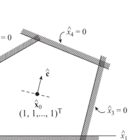
In the internal point methods, we start from a strictly internal point, e.g. x0, so that all the components of x0 are strictly positive (x0>0). When implementing the interior method, an interior starting point that satisfies the constraints is needed.
Quadratic Programming (QP) and the Linear Complementary Problem (LCP)
In the first step, a twisting operation is performed to insert the base and allow it to leave the base. If the last operation results in leaving the base variable z0, the cycle is complete: STOP.