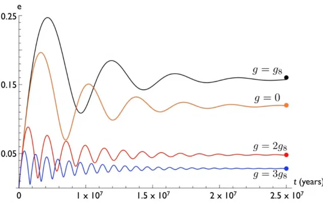
The black curve in the lower graph corresponds to the evolution of the eccentricity of Gliese 436b in the presence of a disruptor. The black curve shows the motion of a fixed point on the Poincaré cross-sectional surface.
Abstract
Introduction
Structural Model & Electrical Conductivity
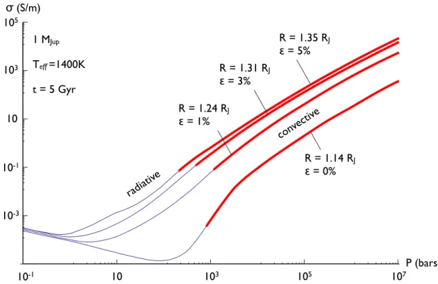
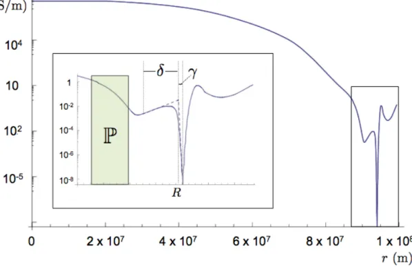
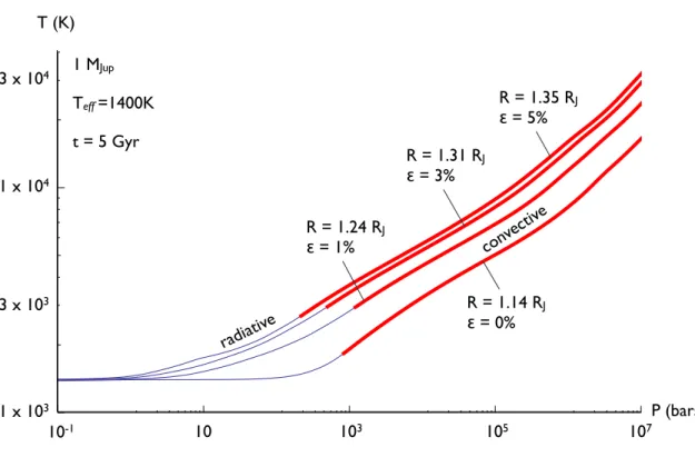
We did not have to explicitly calculate the ionization fractions of H and He, as they are published in the equation of state (Saumon et al., 1995), which we used in our model. Since we are only interested in a part of the planet, inside the atmospheric temperature minimum, we define the model radiusr =Ras the point of maximum conductivity in the atmosphere (P = 75 mbars) and set the outer edge of our model at the minimum conductivity, r = R +γ (P = 30 mbars) .
Analytical Theory
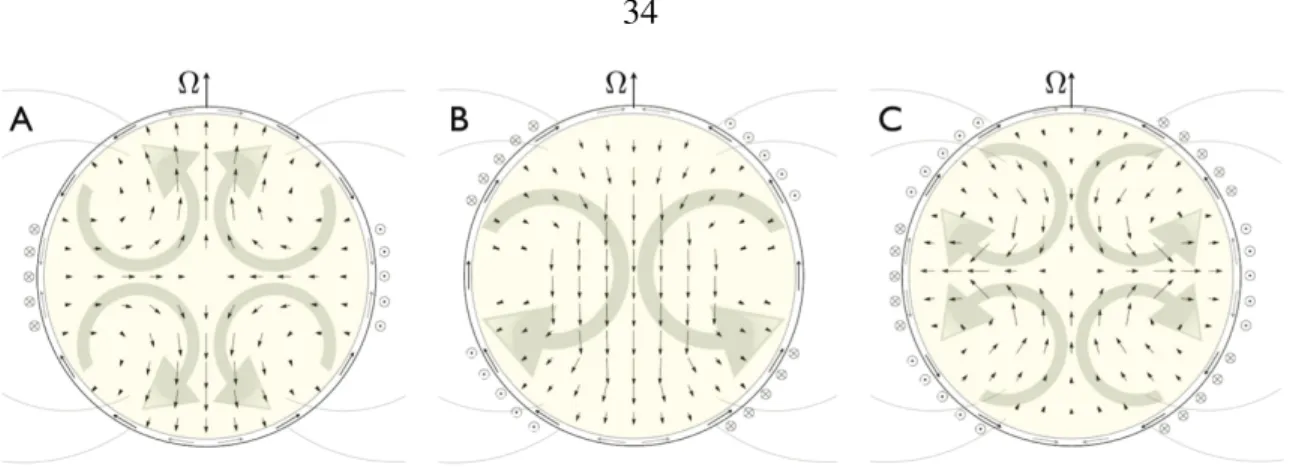
The highlighted region corresponds to the upper convective envelope (100−3000) bars, where most of the internal dissipation takes place. To satisfy continuity, the magnitude of the current density must be constant along its path in the interior.
Model Results
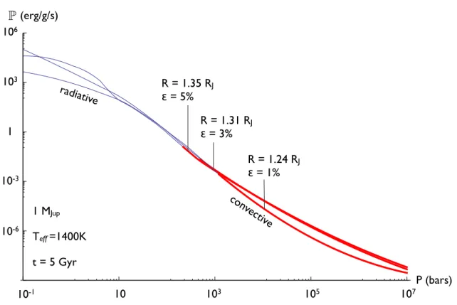
Additionally, to leading order, the dissipation in the atmosphere scales linearly with the thickness of the atmosphere, while the internal dissipation scales roughly quadratically. Here, Rm ~ 15, and the Ohmic dissipation in the atmosphere is again comparable to the insolation.
Discussion
Provided that this size ratio holds in a more dynamical treatment of the problem, it can provide an upper bound on the maximum inflation that can be explained by the Ohmic distribution. While in this paper we have considered only the effects of dissipation in the convective envelope, the intense heating present in the inert layers of the atmosphere may also play an important role in inflation (Bodenheimer, private communication).
Appendix
Although equation (7) must be solved numerically in the interior, towards the center of the planet, where the conductivity can be assumed to be constant, it reduces to Laplace's equation. As a result, we can use the polynomial eigenfunction int(r) =A4r2 near the origin, and A4 is the last undetermined constant.
Abstract
Introduction
In section 2 we consider the energy of the ohmic mechanism and show that at steady state the rate of dissipation is limited by the thermodynamic efficiency of the atmosphere. We conclude and discuss opportunities for future improvement of the ohmic inflation model in section 6.
Work - Ohmic Dissipation Theorem
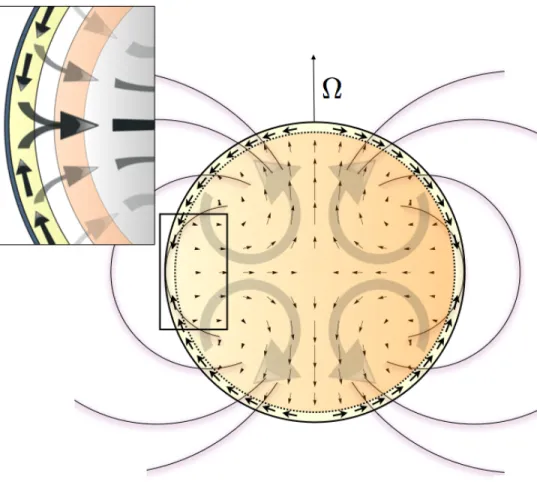
In Section 3, we present a simple model for the damping of the global circulation by the Lorentz force and show that the characteristic efficiency of the Ohmic mechanism is of the order of a few percent. The force or rate of change of energy of the fluid's kinetic energy per unit volume provided solely by the Lorentz force is.
Magnetic Damping of the Global Circulation and the Efficiency of the Ohmic Mechanismand the Efficiency of the Ohmic Mechanism
Note that the Lorentz force is not necessarily antiparallel to the zonal velocity, so the corespodence we use here is only designed to find the effect of the drag. In other words, for most hot Jovian regimes it is reasonable to approximate the effect of the Lorentz force as a Rayleigh drag.
Coupled Ohmic Heating/Structural Evolution Model
This may be important for the ohmic mechanism, since the atmospheric currents determine the induction of the internal current. Thus, the higher, electrically insulating layers of the atmosphere discussed in the previous section would experience very little Ohmic heating.
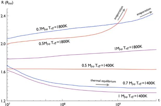
Results: Radial Evolution
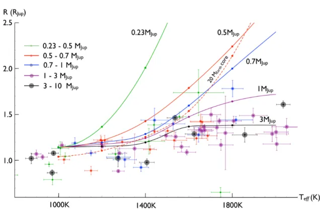
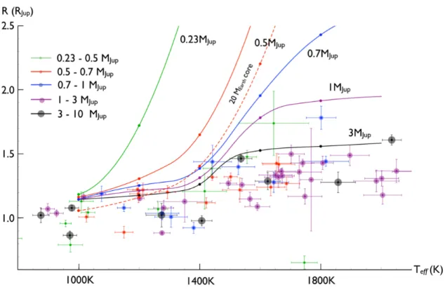
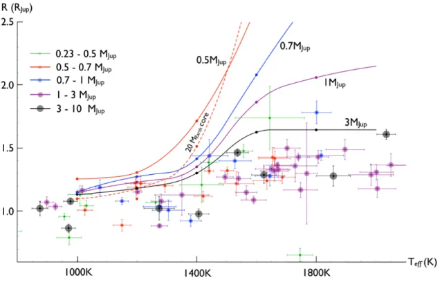
This inevitably leads to Roche-lobe overflow and planet evaporation (Laine et al., 2008). The data masses are sorted between the theoretical curves and are indicated by color and size as shown in the figure.
Discussion
We would like to conclude by discussing future possibilities for improving the model. At the same time, the effect of the induced current on the internal dynamo must be evaluated.
Abstract
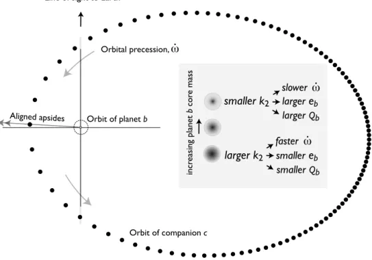
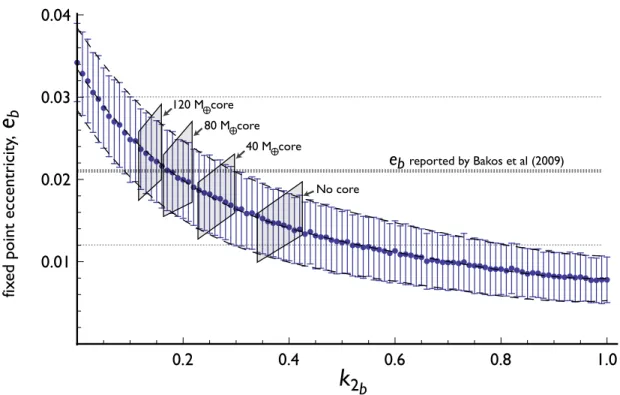
The fixed-point eccentricity of the inner planet is therefore a strong function of the internal structure of the planet. We use an octopole-order secular theory of orbital dynamics to derive the dependence of the inner planet's eccentricity, eb, on its tidal Love number, k2b.
Introduction
We show here that a combination of a tidal-secular orbital evolution model, coupled with models of the internal evolution of the inner planet, can be used to probe the internal structure of the planet and measure the actual tidal quality factor , Q. In Section 2 , we describe the dynamics of a system at a fixed tidal point and we describe the resulting relation between the internal structure of the planet and its orbital eccentricity.
A System at an Eccentricity Fixed Point
The derivations of the planet-induced tidal and rotational precessions are given in Sterne (1939), and are discussed in the planetary context by Wu & Goldreich (2002) and also, extensively, by Ragozzine & Wolf (2009). Tidal dissipation occurs mainly within the inner planet and leads to the continuous lowering of the semi-major axis of the inner planet.
Application to the HAT-P-13 Planetary System
Pure molecular opacities are used in the planet's radiative outer layers (Freedman et al. 2008). In the context of this system, it is important to note that the orbital precession of the planets is quite slow (∼10−3 degrees/year).
Conclusion
As a consequence, we expect the orbital configuration of the system to have evolved somewhat during the current lifetime of the star. The four squares are the approximate areas of the (eb, k2b) space occupied by each of the models presented in Table 1.
Abstract
The results presented here should be useful in further developing a comprehensive model for the formation of the solar system.
Introduction
At the same time, it is also crucial to examine the unobservable aspect of the model, namely the initial conditions. It is worth noting that running simulations of the Nice model to completion is computationally expensive.
Multi-Resonant Configurations
The seminal results of Masset & Snellgrove (2001) showed that locking Jupiter and Saturn in 3:2 MMR can effectively stop the pair's migration. Furthermore, even if Jupiter and Saturn are trapped, subsequent motions can be unstable (Morbidelli & Crida 2007).
Dynamical Evolution
Initial Conditions with Jupiter and Saturn in a 3:2 MMR
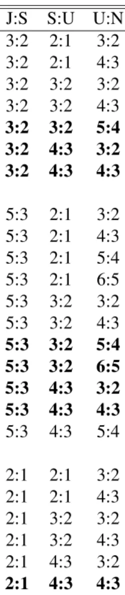
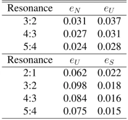
Let us first consider a family of initial conditions, listed in table (1), where Jupiter and Saturn are in a 3:2 MMR. These are the configurations listed in table (1) where both pairs of Jupiter and Saturn and Saturn and Uranus are in MMR 3:2 while Uranus and Neptune are in MMR 4:3 or 5:4.
Initial Conditions with Jupiter and Saturn in a 5:3 MMR
Note that in a scenario where Jupiter and Saturn start in a 5:3 MMR, the instability is caused by crossing the 2:1 MMR, just like in the classical Nice model. Most important, however, are the locations of the planets when Jupiter and Saturn cross the 2:1 MMR.
Initial Conditions with Jupiter and Saturn in a 2:1 MMR
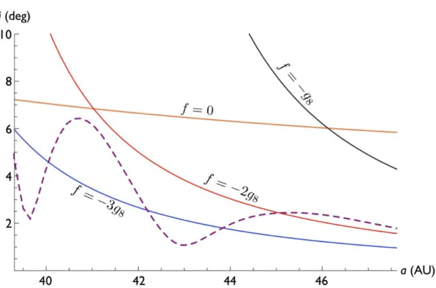
In this case, γ in the argument of the cosine Hamiltonian (5) is replaced by γ0 and its factorp. Note also that all indirect terms in the perturbation function expansion must be accounted for inf(a/a0).
Discussion
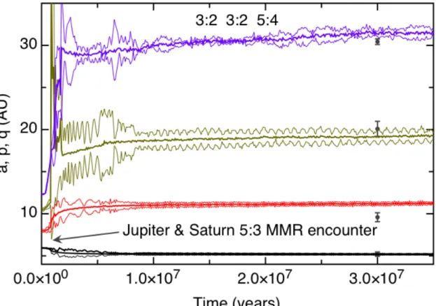
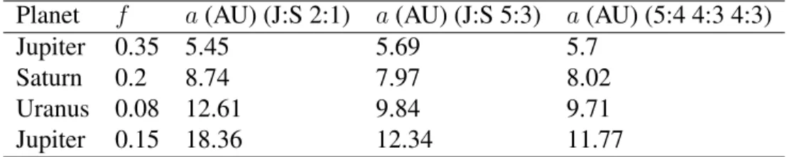
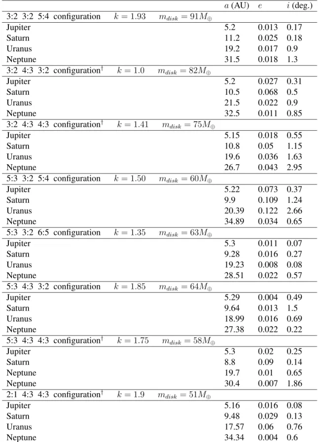
There is definitely room for a broader study of the current problem setting. Orbital elements of solar system analogues resulting from different initial conditions at the end of the dynamical evolution simulations presented in Figs 1–8.
Abstract
We further show that the contamination of the hot classical and scattered populations by objects of a cold classical-like nature has been instrumental in shaping the great physical diversity inherent in the Kuiper belt.
Introduction
The cold population is distinctive from the rest of the Kuiper Belt in a number of ways. Similarly, the size distribution of the cold population differs significantly from that of the warm classical population (Fraser et al., 2010).
Secular Excitation of the Cold Kuiper-Belt
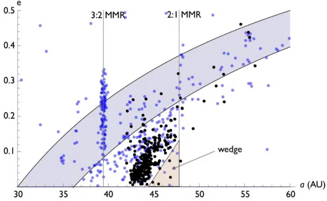
Since we are only interested in the final orbits of the KBOs, we only need to derive the radial part of the solution. Here, we propose that wedge formation is a consequence of secular turbulence.
Numerical Simulations
In the context of these integrations, we can further confirm that the formation of the wedge is due to a significant slowdown in Neptune's precession. Most of the time, Neptune's precession rate exceeds its current value by a factor of a few.
Discussion
The outstanding question of interest is namely planetesimal formation beyond ~ 35AU, given the steep size distribution of the cold classic. 35AU is required to draw a complete picture of the in-situ formation and evolution scenario for the cold classic.
Abstract
Thus, the solar system is one of many possible outcomes of dynamical relaxation and can originate from a wide variety of initial states.
Introduction
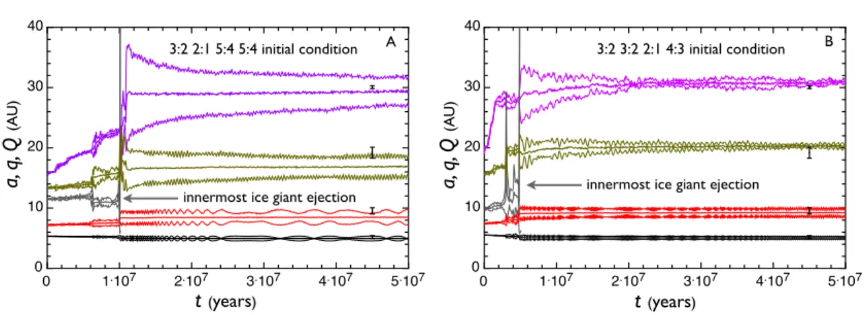
The actual perihelion and apohelion distances of the planets are also shown as black error bars for comparison. In both cases, the inner ice giant is ejected during the transient phase of instability, leaving behind four planets whose orbits resemble those of the Solar System.
Numerical Experiments
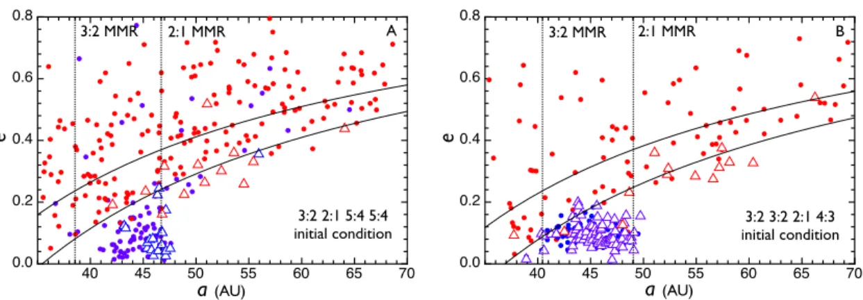
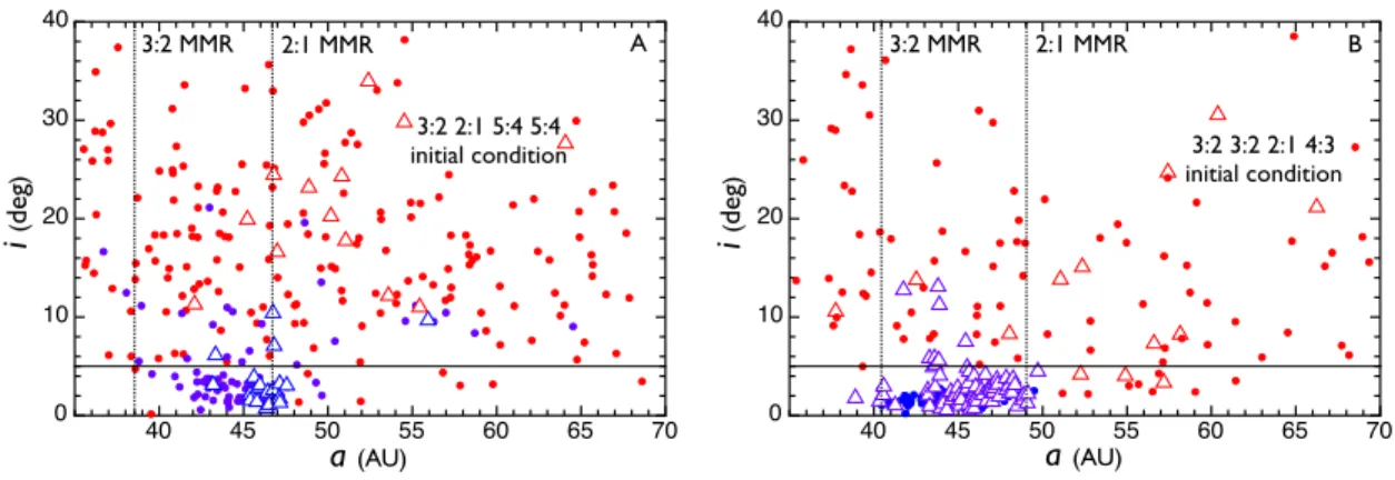
To reduce the already considerable computational cost, the self-gravity of the planetesimal swarm was neglected. In particular, each run was supplemented with an additional disc of massless particles residing in the cold classical region of the Kuiper belt (ie between the final outer 3:2 and 2:1 MMRs of Neptune).
Results
In the 5-planet scenario, the retention of unexcited orbits by the cool population may compromise the launch planet. Consequently, in this simulation, the inner edge of the cold belt is dynamically depleted over the next 500 million years.
Discussion
In a traditional realization of the Nice model, the rate of successful reproduction of the secular eigenmodes is quite low, i.e. the need for an ice-giant/gas-giant encounter in the solar system's orbital history is itself motivation for a 5-planet model.
Abstract
We find a locus for apsidal aligned configurations that are (1) consistent with the currently published radial velocity data, (2) consistent with the current lack of observed transit timing variations, (3) subject to rough constraints on dynamical stability, and which ( 4 ) have attenuation time-scales consistent with the current multi-Gyr age of the star. For the particular example of a perturber with orbital period, Pc = 40 d, mass,Mc= 8.5M⊕ and eccentricity,ec= 0.58, we confirm our semi-analytical calculations with a full numerical 3-body integration of the orbital decay , that includes tidal damping and spin evolution.
Introduction
The possibility that tidal luminosity is observed is prompted by the orbital phase, φ = 0.587, of the secondary eclipse, confirming that the orbital eccentricity is alarmingly high (with a best-fit value of Deming et al. 2007 ). The pseudo-synchronization theory of Hut (1981; see also Goldreich & Peale 1966) suggests Pspin = 2.32d, leading to a 19-day synodic period for planet b. The analysis of Levrard et al. 2007), further indicates that this spin asynchrony of the planet will cause the tidal luminosity to exceed that given by the above formula by a small amount.