Paraj Titum

The quasi-energy gap, in the Born approximation, is shown (cyan) as a function of disorder. b) Propagation egN(r,r0,0) as a function of the total evolution timeTf = NT along the Xdirection, for r0 corresponding to case (I). 99 8.5 Quantized charge pumping in AFAI. pumped charge per cycle in the limit of long times, Q∞, [c.f.

Figure 1.1: Schematic Density of States (DOS) of a band insulator and Anderson Insulator

Born approximation

2π)dG0(E,k0), (1.8) where the self-energy is independent of momentum, k, due to the choice of δ-correlation in the perturbation potential. The imaginary part of the self-energy is related to the mean free time at a particular perturbation strength.

Figure 1.2: Figure shows the Feynman diagrams associated with disorder potential.

Localization due to disorder

In these systems the real part of the self-energy determines the corrections to the parameters of the Hamiltonian. In the next section we discuss the effects of strong disorder on the conductivity of the material.

The localization transition

The two separate cases corresponding to the sign of the β function in the metallic limit are. 1.17). The classification is based on the symmetries of the random matrix: time reversal (T) and spin rotation (S).

Table 1.1: Classification of the different Random matrix ensembles as first proposed by Wigner and Dyson [20, 115]

Summary

We show some of the features of the model in the topological phase in Fig. The real part of the self-energy renormalizes the various parameters in the Floquet Hamiltonian.

Topology in quantum systems

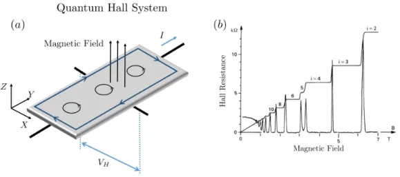
Integer quantum Hall effect

The presence of a magnetic field in the z-direction induces a voltage in the y-direction, the Hall voltage,VH. The quantization of the Hall conductance in a more general arrangement without assuming translational symmetry was demonstrated by Laughlin [62] and Halperin [36].

Figure 2.1: The quantum Hall effect. (a) Schematic set up for the quantum Hall effect

Haldane model for anomalous quantum Hall effect

In the presence of two mass terms, M and ∆, the spectrum is a band gap insulator at zero energy. The pseudospin direction in the band defines a map from the Brillouin zone to the sphere, T2 → S2.

Figure 2.2: Model for anomalous quantum Hall effect [35]. (a) shows the schematic of the tight binding model on a honeycomb lattice

BHZ model for Topological Insulators

In this model we set grid spacing,a= 1. b) The unit vector, ˆd(kx,ky) is a map from {kx,ky}in the FBZ to the unit sphere. Since the Hamiltonian is chosen in the topological phase, the Chern number is non-zero, C =1.

Figure 2.3: Properties of one block of the BHZ model. The Hamiltonian is given in Eq. (2.6) (a) Bulk bandstructure of the model

Disorder and topological phases

The topological nature of the Landau levels has a very important consequence for the nature of bulk states in the Landau levels. This is done experimentally to access the critical exponents of the quantum Hall localization transition.

Figure 2.4: The generic density of states of a 2DEG exhibiting integer quantum Hall effect

Summary

The quasi-energy gap in the band structure depends on the incident polarization of the radiation, given by |V⊥|. In Part II, we study all three models in the presence of disorder.

Periodically driven Topological systems

Floquet-Bloch Theory: Definitions

The eigenvalues () are referred to as quasi-energies, and the eigenfunctions of the Floquet Hamiltonian, defined in Eq. The spectrum of HrF is unlimited; however, we note that in Eq. 3.5), the eigenvalues () of HrF describe the non-periodic evolution of these states as a function of time.

Floquet Topological phases : Haldane model

The attack frequency of the drive, Ω W, where W is the bandwidth of the time-independent band structure. The correction to the energies of non-equilibrium states is obtained by examining the poles of the Floquet Green function.

Floquet topological phases : BHZ model

To obtain the quasi-energy spectrum for the driven system (Eq. 3.22)), we first copy the band structure by translating the original spectrum by Ω as shown in Fig. The Pauli matrices, σ are determined based on the projected quasi-energy bands (see Fig. 3.2) which we name as {|ψ±F(k)i}.

Figure 3.1: Quasienergy bandstructure for the driven honeycomb lattice model for different cases of drive and sublattice pseudospin mass

Floquet Chern insulators with C > 1

For the single resonance case, the Chern number of the truncated HF for M < ∆is. As discussed in Section 3.3, the winding around the north pole, V⊥ (see Eq. 3.27) is necessarily related to the Chern number of the Floquet bands. The Chern number of the band also depends on the polarization of the incident light, as shown in Fig.

Figure 3.4: (a)Winding of V ⊥ (k) on the unit sphere [See Eqs. (3.39-3.41)] as the momentum vector, k varies along the resonance circle [defined in Eq

Floquet TI in Photonic Lattices

The Chern number of bands obtained by radiation of quantum wells with circularly polarized light is ±2. The approximate value of the Chern number for a given polarization angle, θpol = arctan (Ay/Ax), is obtained by calculating C defined in Eq. This system realizes a topological phase as shown by the schematic propagation of a light wave packet at the boundary of the system.

Figure 3.5: Schematic representation of the photonic lattice of the Floquet-Haldane model as realized by Rechtsman et al

Anomalous Floquet Topological phases

In a cylinder geometry, chiral edge states propagate along the upper (green) and lower (yellow) boundaries, only at quasi-energies within the bulk gaps where all Floquet bands have zero Chern number but the winding number 3.45 is non-zero in total gaps. b) The corresponding spectrum, shown as a function of the conserved circumferential crystal momentum component. The bulk spectrum consists of states only with quasine energy = 0, as shown in the spectrum in Fig. The corresponding eigenstates are therefore plane waves, localized on the first row of sites in the A (B) sublattice along the top (bottom) edge.

Figure 3.7: Simple explicit model for achieving the anomalous Floquet topological phase [94]

Summary

In Chapter 5 we first demonstrate the robustness of the Floquet topological insulator in quantum wells to disorder and the survival of the edge modes in the quasine energy gap. This is the driven analogue of the Topological Anderson Insulator (TAI) phase that we examined in Section 2.4. Next, we discuss the different numerical methods to characterize properties of the disordered periodically driven Hamiltonians.

Floquet Born approximation

Numerical methods I: Real-time evolution

To explore the effect of disorder at different quasi-energies, we need the Fourier transform in time of the real-time propagator. 4.11), we Fourier transformed in time to obtain the Floquet Green's function as a function of the quasi-energy. To study the transport properties of the system at a given quasi-energy, we obtain the average transmission probability from x≡ (x,y)tox0≡ (x0,y0) as a function of disorder and quasi-energy. Therefore, the N dependence on the length scale, ΛN(ω), reveals the diffusive or ballistic nature of states.

Numerical methods II: Properties of Floquet eigenstates

4.11), we Fourier transformed in time to obtain the Floquet Green's function as a function of the quasi-energy. The eigenvalues of the Floquet Hamiltonian can be used to study the localization-delocalization transition in this system. The Bott index for periodically driven systems is defined using the eigenstates of the Floquet Hamiltonian.

Summary

The components in the expansion,ΣVx,y,z determine the renormalization of the different components of V≡ (Vx,Vy,Vz). In Figure 8.5(a) we show the cumulative average of the pumped charge per cycle within the limit of long times, Q∞ [cf. 8.7)] as a function of the strength of the disturbance. The random change in the size of the bond is therefore proportional to the strength of the bond itself.

Disordered Floquet Topological phases

Born approximation in resonantly driven BHZ model

The behavior of the full 4× 4 BHZ model in the presence of elliptically polarized light and disorder is subtle. We have the following conditions on the sequence, (i)H(Γ= 0) is the Hamiltonian in the original basis, and (ii)H(Γ→ ∞) is diagonal, and is in the eigenbasis of the Hamiltonian. In Appendix A.4 we outline the procedure to obtain the full eigenfunctions of the system.

Figure 5.2: This figure illustrates the diagramatic representation different terms in the Floquet Green’s function

Numerical Analysis : Destruction of topological order by disorder

Born approximation in the honeycomb lattice

Experimental realization in Photonic lattices

The gauge field, A0, in the photonic system is determined by the helix radius and period. Furthermore, the on-site energies can be varied significantly by changing the refractive index difference of the waveguides relative to the background (which can realistically be varied in the range of 5.0×10−4 by as discussed above). It is important to demonstrate that the strengths of the measuring field, A0, as used here, are directly realizable under experimental conditions.

Conclusions

Floquet conditions are Anderson-localized by the disorder; nevertheless, its edges support chiral edge. states in the main part of the system. The properties of the eigenvalues are given by Random Matrix Theory (RMT) and therefore the eigenvalues experience level repulsion and the level distance distributions obey Wigner-Dyson statistics [79]. We plot the comparison of the IPR obtained from the RG procedure and exact diagonalization in the figure.

Figure 7.1: (a) Bandstructure of the driven system for V z /M = 2, V x /V z = 0.15 in the trivial phase

Floquet Topological Anderson Insulator-II : Floquet-BHZ model 80

Realizing the FTAI using elliptically polarized light

We show that it is possible to detect the presence of the FTAI phase by tuning the polarization of light on a disordered sample. This corresponds to the renormalization of the ellipticity of the radiation, thereby inducing a topological phase at finite perturbation strength, which is the FTAI phase. A consequence of a perturbation-induced topological phase is that a larger fraction of the polarization angles, θ, is topological.

Figure 7.4: (a) Comparison of the Bott index for as a function of the polarization angle, θ for the clean sample and disorder strength, U 0 /M = 1

Conclusions

In this case, the flow of the boundary conditions need not end in a delocalized bulk state. As θx varies, there are avoided crossings in the spectrum, in which the character of the eigenstates changes. The final distribution, PΓ→∞(x), is the distribution of the level differences for all the eigenvalues of the Hamiltonian.

Disorder in Anomalous Floquet phases : The Anomalous

Physical picture and summary of the main results

For localized states, the level space distribution is expected to have a Poissonian shape.

Figure 8.1: The anomalous Floquet-Anderson insulator (AFAI), in a disordered two- two-dimensional periodically-driven system with time-dependent Hamiltonian H (t)

Model

Chiral edge states in AFAI

Moreover, intuitively, if all bulk states are localized, the chiral edge states should persist even within the spectral region of the bulk states. Note that the edge on the opposite edge of the cylinder is wound in the opposite manner, with an edge winding number -nedge. This means that the total edge winding number of the system is zero when the sum runs over all states [52].

Quantized charge pumping

8.4). where the sum goes over all eigenstates that have a peak at one edge of the cylinder, and εj are their corresponding quasi-energy values. When all states are filled near one end of the cylinder, a quantized current flows along the edge. However, the spectrum of states localized near the upper edge, plotted as a function of the current θx passing through the cylinder, clearly shows a non-trivial spectral current.

Figure 8.2: Edge states and spectral flow in the AFAI. a) The parent phase of the AFAI is a clean system without disorder, where all Floquet bands have Chern number zero but the winding number (2) is non-zero in all gaps

Numerical results

Finally, we study the behavior of the system as the strength of the perturbation potential increases. To test this, we simulate the time evolution of wave packets that are initialized in the bulk or near the edge of the system. At this disorder strength, an analysis of the level spacing statistics shown in Fig. 8.3(a) shows that all bulk Floquet bands are localized with a localization length smaller than the system size.

Figure 8.3: Localization of Floquet states in the AFAI as a function of disorder strength, computed for the model presented in Eq

Discussion

The basic idea of the flow equation technique is to preserve the full Hilbert space. The single-particle energy spectrum of the Hamiltonian is obtained from the set of fields. In this section, we discuss the properties of the eigenfunctions obtained from the RG procedure.

Figure 8.7: Floquet spectrum for Thouless’ quantized adiabatic charge pump.

Outlook and Future directions

Simple Example: Spin-1/2 in Magnetic field

Later we investigate the N-site problem by studying the asymptotic behavior of the J distributions under the flow equations. It is clear that whenrmax > Jc the exponent of the initial power law remains unchanged, i.e. the exponent of the power law remains fixed. This figure shows that the method only fails for the highly delocalized part of the phase diagram.

The decay exponent, α for the standard deviation of the distributions remains fixed according to the RG procedure. The RG procedure inspired by the flow equation provides a simple and intuitive description of intermediate-level statistics.

Figure 11.1: Phase diagram of PBRM model, Eq. (11.1), with disordered on-site potential and random hoppings decaying algebraically with range as J i j ∼ |i− 1 j| α

Anderson transitions in power-law random banded matrices

Wegner flow equations applied to Anderson transition

Disordered Wegner’s Flow Equations

At α = 12 the underlying logl contribution cannot be seen due to system size limitations. Let us consider that the number operator at a location k changes as a function of RG time as a result of the evolution. One of the disadvantages of the flow equation technique is that it requires the solution of O.

Figure 12.1: Pictorial representation of the flow equations for the hoppings and fields as calculated in Eqs

Strong-bond RG method

Note that the connectivity distribution function in x - J space typically splits into a product distribution, with a uniform distribution in the x -axis at late stages of the flow. The strong-coupling RG picture also gives the scaling of the transition correlation length. Indeed, we find strong support for all aspects of the RG analysis of the strong coupling from the numerical results.

Figure 12.5: Schematic of the steps in the flow-RG method. The first part consists of finding the bond i, j

Conclusions

The number of sites isNsites = 100 and the total number of steps to diagonalize the Hamiltonian isNsteps= 4950.

Additional numerical results

The validity of the saddle point represents a finite size discontinuity, depending on the size of the systemN. Let be the set of eigenfunctions of the Hamiltonian, ψk(i), where denotes the page index and k the label of the eigenfunction. Characterization of the electronic states near the centers of the Landau bands in the quantum Hall conditions".

Figure A.2: Probability distribution log P log y

Initial Distribution of hoppings

Effect of hoppings on bandwidth

In view of the fact that the power-law exponent of the distribution of Jij does not flow, we rewrite its evolution as

Wavefunction and IPR from RG

Transport properties of non-equilibrium systems under application of light: photoinduced quantum Hall insulators without Landau levels. Anomalous edge states and bulk edge correspondence for periodically driven two-dimensional systems”. Transport properties of Floquet topological superconductors in the transition from the topological phase to the Anderson localized phase”.