Chapter 2
Traction Mechanics
Coordinators: Dvoralai Wulfsohn, Thomas R. Way, Shrini K. Upadhyaya, and William J. Chancellor
Part I. Basic Traction Mechanics
Primary Author: Sverker Persson
Contributing Authors1: Leonard Della-Moretta and Henry Hodges
Tractive effort developed by off-road vehicles has been of interest to people en- gaged in agricultural, forestry, military, and mining operations. Most research con- ducted in off-road traction mechanics has focused on either agricultural or military equipment. From agricultural (and forestry) viewpoints the main emphasis has been on efficiently providing sufficient pull for tillage and transport equipment while reducing or minimizing the damage done to the soil and plants. The prime concern of military research has been the mobility of military vehicles, although more recently some em- phasis has been made towards reducing environmental damage by military equipment.
This review emphasizes agricultural and forestry applications, but other off-the-road uses, including construction equipment and military uses, are also considered. It builds on the pioneering work done by the USDA-ARS National Soil Dynamics Laboratory (NSDL), Waterways Experiments Station (WES), Cold Regions Research and Engi- neering Laboratory (CRREL), U.S. Army Tank-Automotive Command (TACOM), and the National Institute of Agricultural Engineering (NIAE).
Tire development has gone in the direction of larger tires with bigger footprints to support higher dynamic loads, more efficient power transfer, and less damage to the soil. This often means lower inflation pressure (Clark, 1971). Recent advances include the use of low-correct inflation pressures for radial-ply tires which are properly ad- justed to dynamic loads. Rubber track development is another recent significant ad- vance in the traction mechanics area.
Traction devices are mechanical devices producing forces parallel to the surface on which they are supported. They are the components of moving machines that are in contact with the ground. They support the dynamic load of the machine and at the same time produce pull (movement in the direction of travel) and forward motion of
1 Contributions of these authors are identified where appropriate.
Advances in Soil Dynamics Volume 3. S. K. Upadhyaya, W. J. Chancellor, J. V.
Perumpral, D. Wulfsohn, and T. R. Way, eds., 25-58. St. Joseph, Mich.: ASABE. Copyright 2009 American Society of Agricultural and Biological Engineers.
Tractive effort
Direction of travel
Traction space
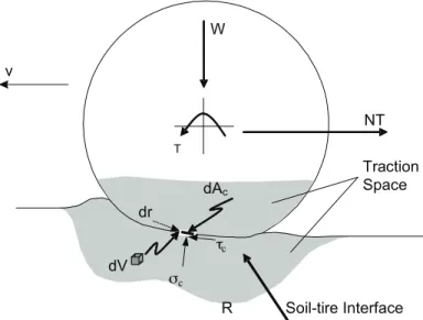
Figure 2.1—Traction space. This consists of all parts of the traction devices and the supporting ground that are affected by the traction forces.
the machine. A transport device is a special kind of a traction device that supports a dynamic load but does not produce any useful pull. The most common traction and transport devices are wheels and tracks, but other devices such as sleds or feet would also fall in this category. Wheels are the most common traction devices, so the follow- ing discussion will be concerned mainly with wheels; tracks will be included only in a few cases. In most cases, however, the general theories and discussions will apply to both. Part IV of this chapter covers tracks in much more detail.
Traction mechanics deals with the interaction phenomena between the soil and the traction device, and the main variables (forces, velocities, power, and energy) in the traction space (fig. 2.1). Traction mechanics also deals with the transfer of forces be- tween a vehicle and the supporting ground. This monograph presents traction mechan- ics in two separate ways: (1) elementary traction mechanics, based on studies of ele- mentary forces acting on every element of the traction space; and (2) gross effect trac- tion mechanics, which considers a single, resultant force acting at the soil-traction interface.
Elementary Traction Mechanics
Elementary traction mechanics deals with stresses and displacements at the inter- face of the soil and the traction device in the traction space. Of special interest are the stresses between one element of the traction device and the element of the soil in di- rect contact with this traction device element (dAc in fig. 2.2), the stress distribution over this element, and associated deformations. Elementary traction mechanics may also include the stresses and deformations inside the soil and inside the traction device (dV in fig. 2.2).
dV
dAc
σc
τc
v
R dr
Traction Space
Soil-tire Interface
T
W
NT
Figure 2.2—Elementary traction mechanics dealing with stresses in contact elements dA and internal body elements dV. An elementary traction theory derives the resultant soil reaction force R and veloc- ity V from the boundary conditions in the contact elements dAc and further relates the contact condi- tions (normal dσc and tangential dτc stresses, and deformations dr) to the conditions in the elements dV of the traction space. The resultant R can in turn be resolved into the net traction, NT, dynamic load, W, and driving torque, T.
The elementary stresses and displacements for a specific element within the trac- tion space will vary with time from the moment when this element enters the traction space to the moment when it becomes no longer influenced by the traction process and exits the traction space. In this chapter, Wulfsohn provides extensive review of the soil-traction device contact region (Part II) and resultant stress distribution (Part III), and Upadhyaya (Part IV) provides analytical expressions for net traction, NT, vertical dynamic load, W, and applied torque, T, if the contact geometry and stress distribution over the contact region are known either from theory or through experiments. How- ever, the interaction between soil and traction device is very complex and it is very difficult to estimate traction parameters such as NT and T using this fundamental ap- proach. Researchers have often resorted to gross effect traction mechanics described below to obtain expressions for traction parameters.
Gross Effect Traction Mechanics
Gross effect traction mechanics describes mainly the relation between the vehicle and the traction device with regard to overall forces and velocities as influenced by traction device dimensions and the soil-traction-device interaction.
The velocities studied in gross effect mechanics are the forward axle velocity, V, of the vehicle and the angular velocity, ω, of the wheel or the drive axle of the track. The forces are the resultant horizontal force component, NT, the vertical dynamic load, W,
Rn
Ψ rt
V ω W
NT
R T
Rt
Figure 2.3—Forces and velocities involved in gross traction mechanics. R = soil reaction; Rn and Rt
radial and tangential components, respectively, of R; T = input axle torque; NT = net traction; V = vehicle forward velocity; ω = wheel angular velocity; W = vertical dynamic load; Ψ = angle of motion resistance of a towed wheel; and rt = the torque radius (Persson, 1967).
and the input axle torque, T, applied by the vehicle to the traction device. The corre- sponding reaction force, R, from the soil acts on the traction device (fig. 2.3). Some typical soil properties may be included in gross effect mechanics.
The vehicle is assumed to be moving with constant linear and angular velocities and the gross effect parameters and their relationships are considered to be independ- ent of time.
The relationship of the variables in the gross effect mechanics can usually be de- termined with sufficient accuracy for predicting vehicle behavior and performance by conducting experiments. Gross effect mechanics is, however, limited when it comes to correlating the tractive performance to soil properties and explaining the performance of a tractive device.
Tractive Power
Tractive power is developed when a vehicle or a device produces horizontal pull in order to move itself, an object, or an implement over a surface. Normally, tractive power considerations refer to machines which move over the surface when they pro-
duce the tractive power; this is the only case that will be treated in this chapter. The case when the vehicle produces only sufficient pull to move itself will be included as a special case: the transport case. Winches and similar devices will not be considered.
Tractive power is basically the product of two physical variables, one being a force or a moment and the other a linear or an angular velocity. Velocities and forces may follow different physical principles and will be treated in the following sections.
Velocities and Tire Radius
Motions of a Traction Device. The motions occurring in the traction space (fig.
2.1) may be studied in two different ways. One group of phenomena relates the actual forward velocity of the traction device (and the vehicle), V, and to the angular velocity of the drive axle, ω. This relationship is discussed in this chapter as a gross effect me- chanics concept. The other group of phenomena involving motion in the traction space describes the relative displacement between individual elements of the traction device and elements of the soil inside the traction space and is classified as the elementary mechanics concept. Velocity as seen as a gross effect phenomenon will be discussed in this section. The discussion of traction device elementary motions will be presented later.
Only steady, straightforward motion, parallel to the supporting surface, in the main direction of vehicle motion and with the vehicle not rotating (no vehicle roll, yaw, or pitch motion) will be discussed here.
Most discussions of traction device motions have considered the traction device (wheel) as being a solid body, where the axle load and the motion from the vehicle enters the tire in the contact between the tire bead and the rim. The corresponding soil reaction force from the supporting surface (ground) comes in as elementary forces (stresses) at the wheel periphery at the outside of the tire belt and tread. However, for modern tires (radial-ply or belted) the bead and the belt are connected by flexible side- walls meaning that the tire cannot be considered to be a rigid rotating body. Many of the relationships derived for the rigid wheel can still be used but with reservations.
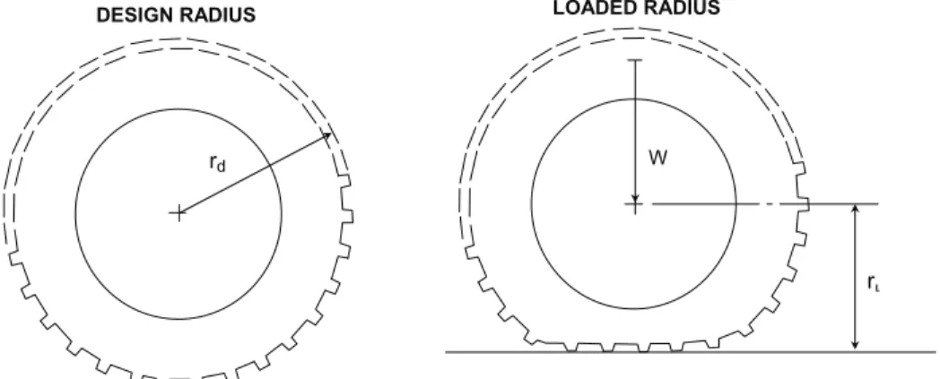
Tire Radius. The radius is the most important descriptive dimension of a tire or wheel. Persson (1995) defines five different measures which are used and needed to describe the radial dimension of a wheel, depending on the purpose for which the di- mension is to be used. These radii are:
• the design radius, rd, for describing the clearance around the wheel;
• the static loaded radius, rι, for axle height and tire deflection description;
• the rolling radius, r, for velocity description;
• the zero-condition rolling radius, r0, used as reference for velocity description;
and
• the torque radius, rt, for force and moment relations.
Figure 2.4 shows the design radius and the static loaded radius. ASAE (1987) as well as most tire specifications give values for the static loaded radius of several agricul- tural tires. The static loaded radius is usually determined on a rigid, flat surface but can also be determined on the actual surface. The rolling radius is described in figure 2.5 and its relationship to r0 is discussed in the next section.
rd
LOADED RADIUS
W
rι DESIGN RADIUS
Figure 2.4—Design radius (rd) and static loaded radius (rι) of tires.
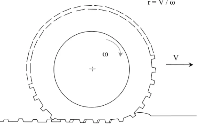
r = V / ω
ω V
Figure 2.5—Rolling radius (r) of a tire.
Torque Radius. The torque radius, rt, as defined by Persson (1967) is obtained by resolving the resultant soil reaction force, R (fig. 2.3) into radial, Rn, and tangential, Rt, components and taking the ratio of applied torque, T, to the tangential component, Rt (i.e., rt = T/Rt). Angle Ψ, the inclination of Rn with respect to the vertical, is given by tan-1(MR/W) for the case of a towed wheel. Consequently, torque radius can be best defined and discussed in connection with the motion resistance, which will be dis- cussed later. Persson (1967) indicated that the value of the torque radius might be es- timated by the zero-condition rolling radius, r0, as determined under conditions of zero net traction. The existence of the torque radius has been sporadically recognized in the literature, but most people using it assume that it exists, do not define it, and do not care about its special nature. The torque radius represents a force or moment relation- ship and not a velocity relationship, as is the case for the rolling radius. There is no logical physical reason to assume that the torque radius is the same as the rolling ra- dius, but this assumption is often made. It should be recognized that the torque radius
is different from the other four radii representations. It would increase clarity and ac- curacy if, when the term “tire radius” is used in traction reports, a statement is made about how the value was defined and determined.
Rolling Radius. The basic physical velocity variables for a traction device in the gross effect mechanics are the angular velocity, ω, of the drive shaft and the forward velocity, V, of the device. The rolling radius, r, is an important variable relating these two basic velocities by the equation
r = V / ω (2.1) where r = rolling radius (m), V = forward velocity (m s-1), and ω = axle (or wheel)
angular velocity (rad s-1).
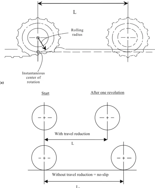
The rolling radius can also be calculated from the distance traveled in one wheel revolution (fig. 2.6):
r = L / (2 π) (2.2a) where L = distance traveled in one wheel revolution (m). This definition, equation
2.2a, is used by ASABE Standards (2008) and many others. Notice that due to tire deformation and travel reduction, L is not normally equal to the wheel circumference.
By these definitions, the rolling radius can take any value from zero for a driven wheel which does not move forward (spinning out) to infinity for a locked (non- rotating) wheel being pulled forward (sliding). (A different definition than in eq. 2.1 has sometimes been used for a braked or sliding wheel.) Additional discussions of the rolling radius will be given when zero-slip conditions for tires and tracks are discussed later.
Further discussions of the rolling radius are given by Steinkampf (1971) and Bailey et al. (1973). The following relationships for rolling radii of an 18.4R38 tractor drive tire were reported by Way and Bailey (1995), with r in m and W in kN:
For an inflation pressure of 41 kP: 1/r = 1.102m-1 + 0.00136m-1kN-1 W (2.2b) For an inflation pressure of 124 kPa: 1/r = 1.057m-1 + 0.00141m-1kN-1 W (2.2c) Center of Rotation
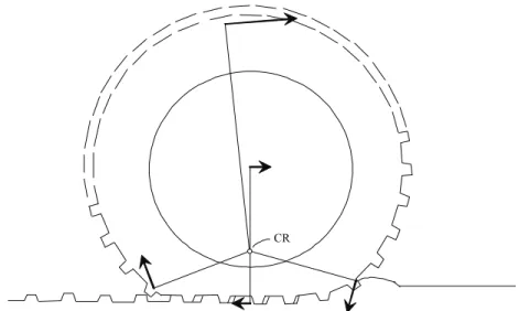
For a moving wheel, one point of the wheel will appear (to a stationary observer relative to a fixed reference system) to be still and the wheel will appear to rotate around this point. The point is called the instantaneous or momentary center of rota- tion of the wheel. It is located a distance equal to the rolling radius directly beneath the wheel center, as shown in figure 2.7.
The center of rotation can be used in describing the motion of any point on the wheel as a rotation around this point, as illustrated in figure 2.7, provided that the point in question is rigidly connected to the hub of the wheel. In tires with radial-ply design the periphery (belt) has a flexible connection to the rim and thus does not fol- low this motion description.
For the theoretical case of a rigid wheel in contact with a solid flat surface with no relative motion between the wheel and the surface at the contact point, the center of rotation is the contact point between the wheel and the surface. For all other cases the
(a)
Rolling radius
Instantaneous center of
rotation
L
(b)
L
Lo
Without travel reduction = no-slip
Start After one revolution
With travel reduction
Figure 2.6—Rolling radius of a tire. (a) Forward travel in one revolution of the wheel, L. (b) Forward travel when the wheel slips, L, versus when it does not slip, L0.
center of rotation is directly beneath the wheel center and at a distance equal to the rolling radius, which can be found only by equation 2.1 or 2.2a. The center of rotation is defined entirely from the velocities and not from the contact forces. It is, therefore, usually not the same as the point of support (discussed in the next section), which is related to the ground reaction contact forces.
CR
Figure 2.7—Instantaneous rotation of a wheel about its center of rotation, CR. The velocity vectors (shown as bold lines with arrowheads) and the respective distances of these vectors from the CR (line perpendicular to the velocity vector that connect to the CR) corresponding to several points on the tire are also shown.
Loss of Forward Motion
The actual forward distance traveled by the traction device (and the vehicle) will be less (or more, in the case of braking) than anticipated from the angular velocity of the drive axle resulting in loss of forward motion and velocity. This fact is given the gen- eral name of “slip.” Two different interpretations of the word “slip” have emerged. In the gross effect interpretation, the actual forward velocity of the vehicle is compared to the forward velocity anticipated from the angular velocity of the drive axle, without consideration of what takes place between the axle and some reference point in the soil outside the traction space. The elementary traction mechanics interpretation (discussed later) views slip as a result of the displacement or deformation of the soil and traction device at the soil-device interface. Slip in the elementary sense varies from point to point in the traction space and is normally present somewhere in all traction cases.
Due to the two different interpretations of the word slip, the term “travel reduction”
(defined in the next section) may be preferable for the gross effect representation of loss of forward motion. However, the common practice is to use “slip” and “travel reduction” interchangeably (ASABE, 2008: ASABE/ANSI Standard S296.5DEC03).
Zero Condition
Travel reduction and slip are measures of a loss in actual distance traveled or for- ward velocity. Before an exact definition of these can be given it is necessary to dis- cuss the reference point or situation where no loss of forward motion is assumed to occur. This traction condition has been given the name “zero condition,” which means a neutral situation where the wheel is not pulling, nor is it being pulled. The situation cannot be defined on a condition of no shear stress in the contact area, because shear stress and displacement always occur at some points of the contact area in any traction
condition for a real wheel. For all real cases, the contact will involve several contact elements which are at different radii from the center of rotation. Relative motion will always occur at one or more of these contact elements and will be of different magni- tude and direction, making a physically defined no-slip condition impossible.
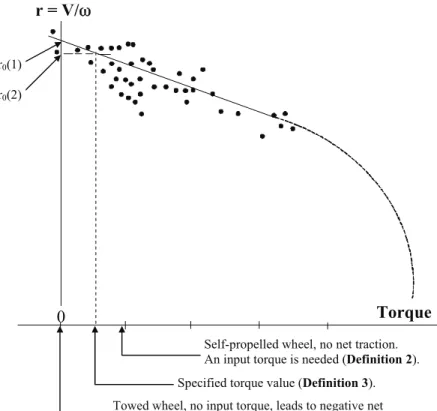
As will be seen later, a definition of a “no-forward-motion-loss” condition as a ref- erence condition is very useful for the description of traction device performance in gross effect traction mechanics. More than one zero condition definition has been used, mainly based on different cases of force or moment transmission between vehicle and traction device. Three alternative definitions used in the literature are given here:
Definition 1: No torque or towed wheel: The zero condition when the wheel has a frictionless bearing and no moment (torque) is transmitted between the traction device and the vehicle. A horizontal force is applied to the wheel at the center, sufficient for overcoming the motion resistance and sustaining the forward motion.
Definition 2: No traction or self propelled: The zero condition when no horizontal force is exerted between the vehicle and the traction device. The traction device is propelled by a torque, applied at the axle and sufficient to overcome the motion resis- tance.
Definition 3: The zero condition between conditions 1 and 2.
Persson (1995) discussed in detail the zero condition and how to find it from traction test data. The main point is that the method for defining the zero condition must be clearly indicated together with the data where it has been used. We hope that some day a general agreement is reached on which method to use.
The forward velocity, V, for a constant axle angular velocity, ω, is influenced by the amount of input torque, T, or the developed net traction, NT. A relationship exists be- tween the rolling radius, r, and the torque, which may be illustrated as in figure 2.8. At low torque values the relationship is linear and can be established by statistical meth- ods. The diagram can be used to illustrate the effect of the three definitions of zero conditions. Each selected zero condition will give a different value for r, the r0 value.
The towed-wheel case, Definition 1, will give the highest r0-value and the self- propelled case, Definition 2, the lowest value. The condition for Definition 3 has been defined from such a diagram as the condition when the specified input torque is equal to the torque needed for self-propelled motion on a rigid surface.
It should be recognized that with this procedure a velocity parameter, the zero con- dition rolling radius, has been defined based on a force relationship. No physical justi- fication for this has been presented and the reason is entirely practical.
As mentioned earlier, each definition will result in a different value of no-slip roll- ing radius, r0, and the no-slip velocity, V0. For this reason all uses of travel reduction or slip data should be accompanied by the definition used for the no-slip condition (ASABE, 2008). A generally accepted agreement is to always use the same definition, which would be very beneficial. ASABE/ANSI Standard S296.5 DEC03 (ASABE, 2008) uses Definition 1 on hard surfaces. Some authors prefer Definition 2 for mobil- ity cases on soft and slippery soil (Freitag, 1990). European authors (Söhne, 1958, and several others) prefer Definition 3 on the actual surface. Definition 1 permits a simple accounting of the energy losses due to travel reduction and motion resistance as de- scribed later.
0 r = V/ω
Self-propelled wheel, no net traction.
An input torque is needed (Definition 2).
Specified torque value (Definition 3).
Towed wheel, no input torque, leads to negative net traction (Definition 1).
Torque
r0(1) r0(2)
Figure 2.8—Rolling radius, r, as a function of input torque. r0 (1) corresponds to Definition 1 and r0
(2) corresponds to Definition 3.
Relationship between Slip, Rolling Radius, and Zero Condition
It is clear from the previous discussion that the magnitude of zero-slip rolling ra- dius, often simply called “rolling radius,” depends on the zero condition. Once the zero condition is defined there exists a unique value of rolling radius that can be de- termined from traction data. Upadhyaya et al. (1988) outlined a procedure for deter- mining this rolling radius from the traction data for the situations where the rolling radius was not explicitly measured or it was not convenient to make such explicit measurements. The procedure is outlined below.
Assume an apparent rolling radius, r', which leads to apparent slip values, s' given by
'r 100 1 V '
s ⎟
⎠
⎜ ⎞
⎝
⎛
− ω
= (2.2d)
If r0 is the “true rolling radius” corresponding to the zero condition, then true slip will be given by
r 100 1 V s
0 ⎟⎟⎠
⎜⎜ ⎞
⎝
⎛
− ω
= (2.2e)
Equations 2.2d and 2.2e can be solved for s' (Upadhyaya et al., 1988) to yield the fol- lowing expression:
s '
s=α+β (2.2f)
where 'r r0
=
β and α = 100 (1– β) (2.2g)
If net traction ratio, NT/W, is given by the following relationship in terms of true slip, NT cs
a(1 e ) W
= − − (2.2h)
then it can be expressed in terms of apparent slip, s', as follows:
⎥⎥
⎥
⎦
⎤
⎢⎢
⎢
⎣
⎡
−
= ⎟⎟⎠
⎜⎜ ⎞
⎝
⎛ β
α
−
−c s′
e 1 W a NT
or NT c cs
a 1 e e W
α − ′
β β
⎡ ⎤
= ⎢ − ⎥
⎢ ⎥
⎣ ⎦
or NT c s
a 1 be W
′ ′
⎡ − ⎤
= ⎣ − ⎦ (2.2i)
where ⎟⎟⎠
⎜⎜ ⎞
⎝
⎛ β
α
=
c
e
b and
=βc '
c , and a and c are empirical traction parameters.2
If equation 2.2i is used as a basis for a nonlinear regression between NT/W and ap- parent slip, s', it will yield regression coefficients, a, b, and c'. These parameters can be solved for α and β as follows:
α = ln(b)/c' (2.2j)
β = 1 – α/100 (2.2k) c = c' β (2.2l) Using eqs. 2.2 g, f, j, k, and l, we can obtain “true” slip, s, and rolling radius, r0, as
follows:
s = (s′ – α)/β (2.2m)
2 This type of expression for net traction ratio is very common for agricultural soils as will be discussed in Part V on traction prediction.
r0 = r'β (2.2n) It should be noted that use of a wrong rolling radius not only leads to a translation
but also rotation of the slip axis in a plot of traction parameters versus slip (cf. eq.
2.2f).
The Travel Ratio and Travel Reduction
Even though the rolling radii, r and r0, are good descriptors of the vehicle velocity a more descriptive variable is the travel ratio, μR, which relates the actual velocity of the traction device and the vehicle to the velocity under zero conditions. The travel ratio may also be described as the ratio between the actual forward travel and the expected forward travel, as shown in figure 2.6. It is dimensionless and the most useful tractive performance parameter for describing velocity relationships.
The most general definition of the travel ratio, μR, in equation form may be based on the rolling radii as
μR = r / r0 (2.3)
where r = actual rolling radius and r0 = zero condition rolling radius as defined earlier.
It has become customary to determine r on the actual surface used for a test series and r0 on a rigid reference surface, but both r and r0 may alternatively be determined on the same surface. The value for the travel ratio will be affected by the choice of reference surface. Other definitions of μR have also been suggested (Koolen and Kuipers, 1983:111). It is useful for describing the actual wheel and vehicle velocity, V, by the equation
V = μR V0 (2.4)
where V0 is the zero-condition velocity for the same angular velocity, ω, as used for V.
V0 may often be the specified vehicle velocity in a given gear. The travel ratio, μR, is basically independent of ω.
Travel reduction, TR, or slip, s, is defined as
TR = s = 1 – μR (2.5)
Note that the value of slip given by equation 2.5 should be multiplied by 100 to obtain slip in percent (eq. 2.2d and e).
Forces on a Traction Device
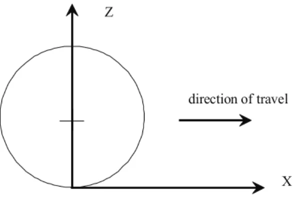
Coordinate System. Several coordinate systems may be used as references for forces and velocities. However, a suitable choice of coordinate system will simplify the representation of the variables and the calculations. The coordinate system used in this section for describing force components is shown in figure 2.9.
The positive X-axis in this system is in the direction of travel of the vehicle and the traction device, which also will be assumed to be parallel to the supporting surface (excluding obstacles and local irregularities). This direction will usually be referred to as being horizontal. The positive Z-axis is defined as being vertically up so it is per- pendicular to the supporting surface.
direction of travel
X Z
Figure 2.9—Coordinate system used for describing forces and velocities of a traction device.
The discussion in this section will be two-dimensional and deals with phenomena in the X-Z plane. Only forces applied to the traction device by the vehicle and the soil will be discussed here, while the discussion of the forces on the entire vehicle will be addressed later. The presentation generally follows ASABE/ANSI Standard S296.5 DEC03 (ASABE, 2008).
Basic Force Components: Counter Turning Moments. The force applied to the vehicle by the traction device can be represented by its two components: (1) the dy- namic load, W, perpendicular to the direction of travel and to the supporting surface;
and (2) the pull or net traction force, NT, acting parallel to the surface. In addition the torque, T, is applied to the axle of the traction device. The weight of the traction device itself is included in these external force components since the gravity force normally acts through the center of the wheel in the same way as the forces from the vehicle (fig. 2.10).
The dynamic load, W, is the instantaneous force on the wheel. It usually varies when the vehicle moves. For clarity, W will be called the dynamic axle load in con- trast to the static axle load which applies only for a traction device at rest and not pull- ing.
The traction device is supported from the ground by the soil reaction force, R. The soil reaction force has to have such magnitude, direction, and location as to be in equi- librium with the forces and moments applied by the vehicle.
The soil reaction force as shown in figure 2.10 is the resultant of all the elementary forces acting between the traction device and the ground. As is the rule for any force, the soil reaction force is fully described by its magnitude, R, its direction, θ, and the line along which it acts, a-a. Note that in the general case a point of action of a force cannot be defined, only a line of action. A further discussion of how to define a “point of action of the soil reaction force” will be presented later. The location of the line of action a-a may be described by (fig. 2.10):
(1) its perpendicular distance from the wheel center, Ltr, (2) its intercept on the Z-axis, z, below the wheel center, or
(3) by the coordinates for an arbitrary point, p, on the line as shown in the figure.
Figure 2.10—Resultant soil reaction force R, which is the resultant of all elementary contact forces acting on the traction device. a–a is the line of action of R, W is the dynamic axle load, T is input tor- que, θ is the inclination of the soil reaction force relative to the vertical and NT is net traction.
The soil reaction force on the traction device must be in equilibrium with the input forces from the vehicle on the wheel and consequently
R = vectorial sum of W and NT (2.6)
tan θ = NT /W (2.7)
Ltr = T / R (2.8)
z = Ltr / sin θ (2.9)
Normally no moment from the ground is necessary for representing the forces in the contact area. An exception to this assumption may have to be made if the wheel is tied or frozen to the ground.
Force Balance: Net Traction. The purpose of a traction device is to produce net traction, NT—a force on the vehicle in the direction of travel—in addition to support- ing the dynamic load. Consequently, the vehicle exerts a force equal to NT on the trac- tion device, opposite the direction of travel. It has been found in traction experiments that when the dynamic load W is increased, the pull or net traction NT will increase in approximately a constant ratio to the dynamic load, if the travel reduction is main- tained at a constant value. Similarly, it has been found that the maximum value for NT that the traction device can produce increases in direct proportion to W. This is an indi- cation that the ratio of the two forces is a characteristic variable for the traction device.
This ratio has been defined as the coefficient of net traction or the net traction ratio, μΝΤ,as
μΝΤ = NT / W (2.10)
Using the net traction concept, the components of the forces acting on the traction device will appear as shown in figure 2.11 (note the sign convention used in the fig- ure). Equilibrium of forces in the horizontal and vertical plane lead to the following equations:
RX = NT (2.11a)
and RZ = W (2.11b)
Equation 2.7, which gives the inclination of the resultant soil reaction force, line a- a', can be written in terms of RX and RZ as follows:
tan-1 θ = (NT/W) = (RX/RZ) (2.12)
Moment Balance: Gross Traction. A certain axle torque has to be added to power the wheel as shown in figures 2.10 and 2.11. This applied axle torque must satisfy the following moment balance equation:
T = R·Ltr = RZ LZ + RX LX (2.13) where LX and LZ are moment arms as shown in figure 2.11.
Figure 2.11―Net traction, NT, developed by a powered wheel.
Substituting equation 2.11 a and b into equation 2.13, we get
T = W·LZ + NT·LX (2.14)
Consequently, the soil reaction force on a powered wheel can be assumed to be the resultant of two soil reaction force components located as shown in figure 2.11 show- ing two parts of the input torque, one due to axle load (W LZ) and other due to net traction (NT LX). Dividing equation 2.14 by LX, we can rewrite equation 2.14 as fol- lows:
L NT L · W L
T
X Z X
+
= (2.15)
T/LX is expressed in force units and is generally defined as gross traction, GT. This force is usually represented as a horizontal force located along the line of action of RX
as shown in figure 2.11. The moment arm LX is sometimes used as an estimate of the torque radius rt, i.e.,
rt = LX (2.16)
From equations 2.15 and 2.16 we have r NT
L · W r GT T
t Z t
+
=
= (2.17)
Unfortunately neither the torque radius, rt or LX, nor LZ are known and they can not be determined from easily measured values. They can be given any value with the only requirement being that they must make RX and RZ intersect on the line a-a. If LX is given a value close to r0 (the zero-condition rolling radius) or rl (the static loaded ra- dius), LZ will get an X-value ahead of the wheel center due to motion resistance. Only a little information about LX is available. Values for r0 or rl are, therefore, often substi- tuted as values for LX. Therefore, GT may be given by
GT = T/r0 (2.18a)
or GT=T/rl (2.18b)
Analogous to the net traction ratio, a coefficient of gross traction or gross traction ratio (μGT), will be defined as
μGT = GT / W (2.19)
Motion Resistance. Equation 2.17 can be rearranged to obtain the following ex- pression:
NT r GT
L · W
t
Z = − (2.20a)
The term on the left side of the equation is equal to the difference between gross trac- tion (GT) and net traction (NT) both of which are in the horizontal direction. This
quantity which is horizontal in direction and expressed in units of force is termed the motion resistance, MR. Therefore,
MR =
t Z
r L ·
W = GT – NT (2.20b)
Since LZ and rt are not known, MR can not be directly measured except in the fol- lowing two situations, the towed wheel and the self-propelled wheel.
For a towed wheel, input torque and therefore GT are equal to zero. Consequently, from equation 2.20b MR becomes:
MR = –NT (2.20c)
Figure 2.12 is a schematic diagram of the towed wheel. Note that the resultant soil reaction, R, passes through the wheel center in this case since there is no input torque.
Moreover, MR is equal to a measurable force, NT = –RX in this case.
For a self-propelled wheel, NT is equal to zero and equation 2.17 yields
MR = GT
r T r T
t MR
t = = (2.20d)
From equations 2.20b and 2.20c, we have
RZ R
MR = RX
W
NT
Figure 2.12—Motion resistance, MR, of a towed wheel. W is the dynamic load and R is the tire-soil reaction force.
t MR t
Z
r T r
L ·
MR= W = (2.20e)
or W·LZ = TMR (2.20f)
or W
LZ =TMR (2.20g)
Figure 2.13 shows the schematic diagram of a self-propelled wheel with zero net trac- tion and an input torque, TMR, which is equal to the soil reaction force, R·LZ. Note that soil reaction force, R, is equal to the dynamic load, W, in this case.
For the case of a powered wheel, which has an input torque, T, and produces a net traction, NT, the motion resistance results in a higher value of the input torque, T, than had been necessary if there had been no motion resistance. However, in this case, there is no way to distinguish by measurement between that part of the input torque which is due to the developed net traction and that part which is due to the motion resistance.
Nor can a separate motion resistance force be distinguished from the other horizontal soil reaction forces by measurements or other observations. In spite of this, it has be- come customary to define a motion resistance on the basis of equation 2.20b, i.e.,
MR = GT – NT (2.21a)
W
TMR
R
LZ
Figure 2.13—Motion resistance, MR, of a self-propelled wheel with zero net traction. TMR is the input torque, R is the soil reaction force, and LZ is the distance between the line of action of R and the verti- cal axis through the wheel center.
Similar to net and gross traction ratios, a motion resistance ratio or a coefficient of motion resistance is defined as:
W MRR=MR
=
ρ (2.21b)
where ρ = motion resistance ratio.
Equation 2.21a is often rearranged and written as:
GT = NT + MR (2.21c)
A different way for defining GT and MR has also been presented based on the ele- mentary contact stresses between the wheel and the supporting surface which will be discussed later. The gross traction, GT, has been assumed to be equal to the sum of all the horizontal components of the tangential component of the elementary forces and the motion resistance the sum of the horizontal components of the radial component of the same elementary contact forces. The sum of the vertical components of the same elementary contact forces should be equal to the axle load. Unfortunately, this ap- proach cannot be applied to the towed wheel or the self-propelled wheel. Therefore it is debatable which elementary contact stress components should be included in GT and MR, respectively. Due to the complicated nature of the contact stresses, the appli- cation of this method becomes difficult to use and not very accurate.
An alternate and often preferable approach is to interpret motion resistance from energy considerations. This approach will be discussed later in this section.
It should be noted that for all cases (towed, self-propelled, and powered), the verti- cal soil reaction force at the contact region Rz is located ahead of the wheel center line (i.e., line of action of dynamic load, W). This requirement also applies to two-axle tractors. Figure 2.14 illustrates the effect of motion resistance on the load distribution
LZR
RZR RZF
LZF
Figure 2.14—Soil reaction forces on a two-axle vehicle with motion resistance.
between front and rear axle for a two-axle tractor. The fact that soil reaction forces on the front (RZF) and rear (RZR) wheels are caused to move forward of the front and rear axle centers, respectively, will result in a counterclockwise moment on the tractor.
This moment leads to an increase in the rear axle dynamic load and a decrease in the front axle dynamic load as compared to the values that would have applied for a static vehicle on a non-deformable surface. For a vehicle with a short wheelbase the effect may be substantial.
Location of the “Point of Support”
For many occasions, e.g. calculating the load distribution between wheels of a moving and pulling vehicle supported by several wheels, the determination of a point where the soil reaction force is transferred to the vehicle at each wheel is more useful than the lines of action.
Fundamentally, the location of the soil reaction force is given by the location of its line of action, with any point on this line being equally justified as a point of action for the force. When the traction of the traction device changes, the line of action of the soil reaction force will also change. If these lines would always intersect at one point, this intersection point would be a natural choice for the point of support. This may happen for a rigid wheel on a rigid surface. Unfortunately, in most other cases with non-rigid wheels on a soft surface the action lines do not intersect at the same point when the net traction changes, due to the changing contact stress distribution. Another definition must be found, remembering that in a physical sense a real “point of sup- port” does not exist.
Based on previous discussion of motion resistance and torque radius, a simple me- thod of defining a “point of support” can be used for both the net traction and the gross traction method of describing soil reaction forces in the X-Z plane. The horizontal components of the soil reaction force are assumed located at the distance rt below the center of the wheel. This will cause the vertical component RZ to fall a distance LZ
ahead of the center of the wheel. The two distances rt and LZ define a virtual “point of support” for the wheel. Locating the soil reaction force in the point (X = LZ, Z = –rt) will put it on the proper line of action and satisfy both force and moment equilibrium equations for the wheel.
In the general case of varying net traction, the distance LZ is expected to be a func- tion of the net traction. This means that when the net traction changes a fixed value for LZ and rt will place the point on the line of action only in one specific case and will place it beside the line in all other cases. For practical use when the representation should be as accurate as possible in most cases, the value should be chosen to give the least possible average deviation from the lines. The case when LZ = 0 (i.e., the “point of support” is directly beneath the wheel center) is not a good choice, because it does not apply for the situations where the net traction is small or zero.
However, it has been shown (Persson, 1967) that the distance LZ is a more gener- ally useful description of rolling resistance than the motion resistance ratio ρ. LZ is, for instance, often independent of the radius of the wheel when the load is constant.
Therefore, the motion resistance ratio may be expressed as
ρ = LZ / rt (2.22)
With a constant LZ, equation 2.20g often reflects fairly well the effect of wheel radius on the coefficient of motion resistance.
Due to the general lack of knowledge of rt, application of the above methods will normally require an assumption about one of the variables. If LZ is known, rt can be calculated from equation 2.23. Eventually more information about LZ may become available but until then an assumption about rt itself will likely have to be made. The first such assumption may be that rt = r0, the zero-condition rolling radius, and the sec- ond one may be that rt = rl, the static loaded radius.
When a tire produces high net traction and absorbs high torque on a hard surface the tire will deform considerably, bringing the tire center to the rear relative to the con- tact area and closer to the surface. This may have the effect that the value for LZ, cal- culated according to equation 2.20g, will be “unnaturally” large. These equations will give correct values for T even with such “unnatural” LZ values. In general, a consistent use of the same definitions will yield correct results even when the values for r0, LZ, and ρ are approximated.
Consequently, using the net traction concept the torque necessary to move the wheel will have two components, one corresponding to the net traction and the other corresponding to the dynamic load, which can be expressed as (cf. eq. 2.14)
T = NT·rt + W·LZ (2.23)
The first part of the torque, NT·rt, may be considered a useful torque producing useful traction, while the second part, W·LZ,represents a torque loss necessary for overcoming motion resistance energy losses. This agrees with equation 2.20e for the self-propelled wheel where the torque is needed only for overcoming motion resis- tance and no net traction is produced or needed. When equation 2.23 is applied to the transport wheel along with equation 2.20e, fig. 2.11 gives NT = –W·LZ/rt = –MR or NT = –ρ W, as expected.
Sometimes this illustration is also used to explain the effect of soil resistance on the wheel. The wheel is said to require additional torque because it is always in a situation equivalent to “rolling uphill” due to the location of the point of support ahead of the wheel center.
Power Considerations
3Tractive or Output Power
The useful power produced by the traction device and transferred to the vehicle is the product of the net traction, NT, and the wheel (vehicle) forward velocity, V. This is called the tractive power, TP, of the traction device:
TP = NT·V (2.24)
Note that the tractive power of a tractor (vehicle) will be defined later.
3 This section was written by Sverker Persson based on notes provided by Leonard Della-Moretta.
Input Power
To produce this power the torque, T, has to be applied to the wheel and the wheel turned at the angular velocity of ω. The input power IP is consequently defined as
IP = T·ω (2.25)
IP can be calculated also from the equation
IP = GT·V0 (rt / r0) (2.26)
This equation can be derived by substituting (GT·rt) for T from equation 2.17 and V0
= r0ω. Further assuming r0 = rt gives the simpler equation
IP = GT·V0 (2.27)
Tractive Efficiency
The ratio of the tractive power (output) to the input power is expressed by the per- formance parameter tractive efficiency as
= ω T
V ·
TE NT (2.28)
Tractive Power Ratio
The tractive power ratio is a non-dimensional tractive performance variable defined for the purpose of finding optimum traction device performance. This tractive power ratio is defined as
TP W ·V0
= TP
μ (2.29)
The numerator in this equation is a power quantity. The denominator is the product of dynamic axle load and theoretical forward speed, V0, that makes tractive power ratio a dimensionless number. The usefulness of this non-dimensional parameter will be dis- cussed later.
The tractive power ratio can also be written as
μTP = μNT μR (2.30)
showing the dual influence of net traction (force) and travel ratio, μR = V/V0 (velocity) on the tractive power developed by the tractor.
By computing the tractive power ratio from test data taken over a range of net trac- tion levels the user of the traction device can determine the operating conditions (level of net traction applied) to obtain the maximum power that a given traction device can transmit, at given levels of dynamic load and drive axle angular velocity, under any specific set of soil-traction-device interface conditions. In effect, this parameter takes account of the simultaneous effects of slip energy losses and motion resistance energy losses. For most cases this maximum power condition represents the peak economic value of the traction device to the user under the specified conditions.
Figure 2.15—Power distribution in a powered wheel.
Energy and Power Losses in Traction
The input power is always larger than the output power due to energy losses in the traction space. The difference may be represented by two kinds of power losses, PL1 and PL2 (fig. 2.15).
The relationship between the output tractive power and the input power may be ex- pressed symbolically as
TP = IP – PL1 – PL2 (2.31a)
The power loss PL1 will be called the slip loss and defined as
PL1 = IP·TR (2.31b)
where TR is the travel reduction or so called “slip”, S, and the power loss PL2 is called the motion resistance loss and defined as
PL2 = MR·V (2.31c)
The correctness of equation 2.28 can be found by substituting NT + MR for GT from equation 2.13 and V + V0·TR for V0 from eqs. 2.4 and 2.5.
The energy and power balance in the conversion of input power to tractive power is illustrated in figure 2.15 and may be expressed in words as (tractive power) = (input power from the transmission) – (slip power loss) – (motion resistance power loss).
Figure 2.15 illustrates graphically how the input power may be divided between the tractive power and the two power losses using eqs. 2.27 and 2.28 and gives a simple interpretation of the power losses. As shown, PL1 represents that velocity part of the input power, which does not result in forward velocity, i.e., the slip power loss. PL2
represents the torque part of the input power, which does not result in net traction, i.e., the motion resistance power loss. This discussion is based on the definitions of GT and MR described earlier.
For the case of the self-propelled wheel with zero net traction (as depicted in fig.
2.13) the power-loss quantity PL2 is
PL2 = TMR ω (2.32a) Since, from fig. 2.13,
TMR = W·LZ (2.32b)
PL2 = W·LZ ω (2.32c)
Thus, from figure 2.15 it can be seen that
V
L · W V T V
2
MR PL MR Zω
ω=
=
= (2.32d)
where ω/V = 1/r0, and r0 is the rolling radius for the zero-net-traction condition of a self-propelled wheel, while V = V0 for this same condition. In this case the motion resistance, MR, is computed as having units of force: a force of magnitude MR, which when applied at velocity V in the direction of motion would exactly compensate for power loss PL2. There is, however, no basis for assuming that a force of magnitude MR reacts with the traction device at any particular position or in any particular direc- tion.
The division of the total energy loss may be made in other ways than shown above but this division seems to be the simplest.
Power Distribution in a Tractor
Agricultural tractors use their power mainly as tractive power in pulling imple- ments in the field. Figure 2.16a illustrates how the engine power for a normal rear- wheel-driven four-wheel tractor is being distributed through the tractor. The useful power delivered to the implement is called the drawbar power of the tractor (1 in fig.
2.16). In addition, power is needed for overcoming the motion resistance of the tractor (2r and 2f in the figure) and for covering the slip losses between the ground and the traction devices (3). Before the engine power (5) reaches the drive wheels, transmis- sion losses (4) are encountered before the power is delivered to the traction device as input power (6). A more specific representation of these different amounts of power is given in the Sankey diagram, figure 2.16b.
The drawbar power DP delivered by a tractor to the implement at the drawbar or any other point of attachment is the product of the horizontal component of the draw- bar pull, H, and the forward velocity, V:
DP = H·V (2.33a)
Tractive Efficiency of a Tractor
The tractive efficiency of a traction device was defined earlier. Similarly a tractive efficiency for the tractor may be defined as:
(drawbar power) / (axle power developed to provide this drawbar power)
(a)
5 4
6
2f
2r 3
1
(b)
5 6 7 8 1
4 3 2f 2r
Figure 2.16―(a) Power distribution in a tractor and (b) Sankey diagram of power flow. 1 = drawbar power, 2 = rolling resistance power (2f = front, 2r = rear), 3= slip power loss, 4 = transmission loss, 5 = engine power, 6 = input power to traction device, 7 = gross tractive power, 8 = net tractive power.
As can be seen from the Sankey diagram, the tractive efficiency for the tractor is con- siderably less than the tractive efficiency for the traction device because the drawbar power of the tractor may be less than the net traction power from the traction devices if the tractor has non-powered wheels.
It should also be observed that the engine power which is actually being used is normally less than the maximum power the engine can develop because the engine seldom operates at the speed and torque associated with the conditions at which max- imum power is developed.
Tractive Power Variations
Assuming a constant transmission efficiency for a given level of engine output, the input power to the traction device should be the same for all gears. Theoretically this would mean that the drawbar power would be the same in all gears. A low gear would theoretically give a high gross traction force and a high gear a low gross traction as shown in figure 2.17. This will not be true due to the power losses.
A low forward speed will require a high drawbar pull in order to fully use the input power. This will result in high slip power losses. At a high forward speed the power loss for overcoming the motion resistance takes a larger portion of the input power.
For a well designed tractor the power losses are at a minimum at an intermediate for- ward speed and, consequently, the drawbar power and the tractor tractive efficiency
Intermediate gear
Pull Low gear High
gear
Drawbar power
Figure 2.17―Effect of pull on drawbar power in different gears.
are at a maximum (fig. 2.17). As discussed earlier regarding the tractive power ratio, the maximum tractive power does not normally occur at the same speed and pull as maximum net traction or maximum tractive efficiency. This distinction should be ob- served when selecting the size of implements for a tractor, and when selecting tire equipment and weighting for a tractor of a given power level.
As a general rule, a heavy tractor with low-slip traction devices, as for instance a crawler, has its optimum drawbar power at a low forward velocity. A light tractor on a surface where the coefficient of traction is low and the coefficient of motion resistance is low, has its maximum power at a high forward velocity. Under all circumstances, the highest forward velocity should be kept below a value for safe tractor operation.
The drawbar pull will be limited to the value where the drive wheels will spin out, i.e., travel ratio = 0.
The above discussion was made assuming a constant transmission efficiency. Some modern transmissions, however, have a marked peak efficiency at a certain gear ratio.
The most favorable operating speed for the tractor, should, therefore, be selected con- sidering this factor as well.
For transmissions with fixed gear ratios the optimum utilization of maximum en- gine power can occur at, or close to, only one specific forward velocity for each gear.
At other velocities the engine speed must be lowered and the available engine power become lower. The transmission, thus, has the effect of permitting the possibilities of having maximum tractive power available at all forward velocities.
It should also be recognized that tractors in practice operate with smaller imple- ments and at lower speeds than could actually be handled, resulting in even lower uti- lization of available engine power.
Tractors are normally officially tested in conjunction with the Nebraska Tractor Test Laboratory or at another Organization for Economic Co-operation and Develop- ment tractor test center on a test track with a favorable traction coefficient and with a well selected weight distribution of the tractor. The drawbar power figures available
from tests done in conjunction with the Nebraska Tractor Test Laboratory should, therefore, be considered as maximum values that can only seldom be achieved during agricultural conditions. A tractor in normal field work operates on a surface with a lower coefficient of traction and with a higher rolling resistance than is the case for these test tracks. It may not be ballasted in the most efficient way. The drawbar pull is not constant but varying. Therefore, the average drawbar pull has to be selected to be less than the maximum value. The average drawbar power developed by a tractor in the field is, therefore, considerably less than found in reports of tests done in conjunc- tion with the Nebraska Tractor Test Laboratory. A figure of 60% of the power level found in tests done in conjunction with the Nebraska Tractor Test Laboratory should be considered a favorable value and the value is often considerably below 40%.
Burt and Bailey (1981) presented tables and curves of the effects of combinations of dynamic load and inflation pressure on net traction and tractive efficiency. They can be used for evaluation of tractive power ratio.
Traction Device Performance Parameters
4Optimum Tractive Device Performance
Measures of performance are needed for the selection, design and use of traction devices for their use on a vehicle. The main points of interest in discussing the per- formance of a traction device are:
• How much power can it develop under given circumstances?
• How much pull or net traction can the device produce?
• How much torque must be provided at the drive axle?, and
• What forward speed will result for a given angular velocity of the drive axle?
Parameters answering these questions will be defined as the principal performance parameters.
The criteria used for determining which factor should be considered for expressing optimum performance and what values the selected parameter should have in order to be considered as optimum may vary from one application to another. One group of criteria involves maximum drawbar pull, maximum tractive power, and maximum tractive efficiency. Another group includes limits on tire width due to row crop spac- ing, and tire diameter, for crop height clearance. A third group concerns soil damage and compaction, crop damage, tire sinkage, and rut depth. Considerations must be given to tire cost, tire wear, and vehicle cost. Vehicle steering and vehicle dynamic behavior are other factors of concern.
How to Present Tractive Performance Measures
Tractive performance of a traction device can be determined through tests. The in- dependent variables, the magnitude of which can be chosen at the discretion of the designer or researcher, are usually tire configuration, soil condition, dynamic load on the tire, and rotational speed of the drive axle (or equivalent). The dependent vari-
4 This section was written by Sverker Persson based on notes provided by Leonard Della-Moretta.
ables, which are measured and recorded, are the net traction, the required torque on the drive axle (or equivalent), the forward velocity, and sometimes the sinkage.
The test results are transformed for greatest and most general usefulness into non- dimensional tractive performance parameters as defined earlier. The tractive perform- ance of the device can be completely described by a set of three such parameters, for instance, μNT, ρ = MR/W = μMR, and μGT. The zero-condition rolling radius r0 should also be determined and specified. Other parameters such as tractive efficiency can be calculated from these three basic parameters as well as the velocity variables as de- scribed previously.
Test results indicate that characteristic changes in tractive forces (GT, NT, and MR) can be related to wheel and forward speed of the vehicles. The simplest and most ac- curate presentation of the measured relationship is by plotting the variables against each other in diagrams. The common way of doing this has been to use the travel re- duction as an independent variable and to plot the net traction and the torque as de- pendent variables (fig. 2.18). This is, however, not the best way when finding some optimum points in the relationship for design and comparisons, even when the non- dimensional equivalents are used. A mathematical expression for the relationship, for instance as an equation μNT = f (μTR), is very desirable. Unfortunately, the relationship cannot easily and accurately be represented by an equation, even though some equa- tions represent a fair approximation for certain cases. A review of such traction predic- tion equations will be presented later in Part V of this chapter.
0 .6
0 .4
0 .2
2 0 4 0 6 0 8 0 1 0 0
T r a v e l re d u c ti o n μM R
μN T
T E
0 0 . 0
Figure 2.18―A typical plot of net traction ratio, μNT, motion resistance ratio, μMR, and tractive effi- ciency, TE, as a function of travel reduction or slip.
μTR
TE
μGT
μNT
0.2 0.4 0.6 0.8
μMR 0.2
0.4 0.6 0.8 1.0
Figure 2.19―Tractive characteristics of a 13.6-28 tire at 128 kPa inflation pressure plotted as a func- tion of the net traction ratio.
The diagrams or equations do not immediately give the performance information for cases where an optimum size of an implement should be selected for a given trac- tor. For such purposes, it is more useful to use diagrams, where the coefficient of net traction (representing the pull) is the independent variable and gross traction ratio (representing the torque) and travel ratio (as the speed) are the dependent variables, as shown in figure 2.19.
The traction performance parameters are influenced by soil conditions, design fac- tors and operational factors. These influences are discussed in Part VII of this chapter.
Representative Performance Points
The traction test data presented in a diagram cannot be used as such for vehicle de- sign and calculations of tractive power. For such calculations, specific points have to be selected from the diagrams, each point corresponding to one specific condition and giving a specific set of three performance values. Different points may be selected depending on the purpose of the calculation. The main interest is usually tied to find- ing the net traction at which the maximum tractive power or the maximum tractive efficiency occurs. The maximum tractive efficiency occurs at one specific condition of operation and the maximum tractive power ratio always at a different condition. A decision must be made for which conditions the performance parameters shall be se- lected: for maximum pull, for maximum efficiency or for maximum power output.
The net traction has at least a practical if not an absolute maximum. For many ground surfaces the absolute maximum pull occurs at 100% travel reduction. Since this is of little practical value the maximum pull is often defined as the pull at the point
Figure 2.20―Net traction ratio corresponding to various operating points for a traction device.
of maximum permissible travel reduction (Point 3 in fig. 2.20). For normal field con- ditions and bias-ply tires, the maximum permissible travel reduction is often set at 25 percent travel reduction; for adverse conditions sometimes higher, up to 50 percent or more. On hard surfaces the maximum permissible travel reduction should probably be set at 10 to 15 percent considering the wear of the tires. The parameters for maximum net traction can be used only for setting the limit of operation, beyond which the vehi- cle should not or cannot be used.
The point of maximum tractive efficiency occurs at a net traction considerably low- er than the maximum pull (Point 1 in fig. 2.20). It often occurs at such a low pull that it cannot be used practically for vehicle design calculations, because it would result in selection of excessively heavy tractors for a given implement size in operations which require a fairly low forward speed.
A third significant tractive performance point has been suggested by Persson (1967, 1991) as the point at which the maximum value of the tractive power ratio, μTP, takes place. The calculation of μTP, is given as
μTP = (NT·V) / (W·V0) (2.33b) This ratio defines the conditions where maximum tractive power is produced by a traction device when it has a given vertical dynamic load and is driven in a given gear and at given engine speed. Operating the traction device at this condition (point 2 in