Finally, this book contains an appendix that supplements the main parts of the book with a detailed discussion of supplementary topics. This book is not intended to be simply a collection of algorithms that can be immediately applied to various problems that may arise in Computational Physics.
Some Basic Remarks
- Motivation
- Roundoff Errors
- Methodological Errors
- Stability
- Concluding Remarks
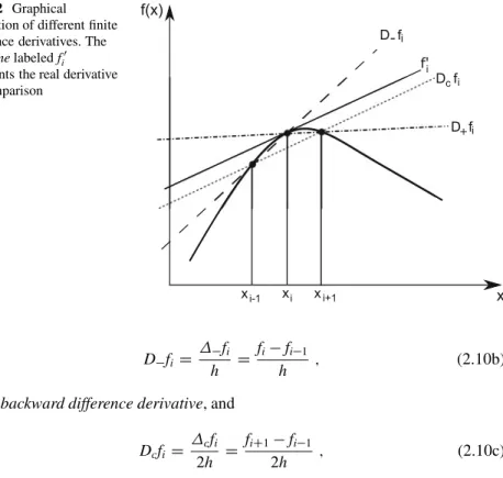
Before continuing our discussion of rounding errors, we need to introduce the concepts of absolute and relative error. Whenever an arithmetic operation is performed, the errors of the variables involved are transferred to the result [15].
Deterministic Methods
Numerical Differentiation
- Introduction
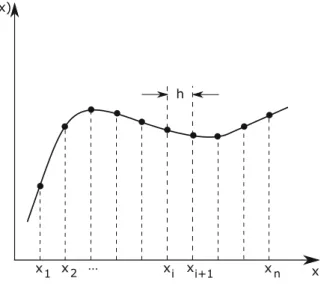
- Finite Differences
- Finite Difference Derivatives
- A Systematic Approach: The Operator Technique
- Concluding Discussion
We can write these operators in terms of the forward and backward difference operatorsCandof Eq. However, it appears that the expansion (2.27) in terms of the central difference c does not use the grid optimally because it only contains odd powers ofc.
Summary
Problems
For the second order correction of the central difference derivative take the term proportional toıc4in Eq.
Numerical Integration
Introduction
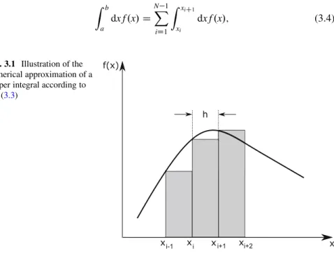
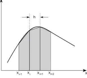
Rectangular Rule
On the other hand, if the method considers endpoints, it is called a rule of closed integration. 1In this context, the intermediate position xiC1=2 is understood as a true grid point. If, on the other hand, the value of the function fiC1=2 is approximated by fiC1=2, equation 2.29), the method is called the trapezoidal rule.
Trapezoidal Rule
12fi00C So we see that the error caused by the trapezoidal rule is similar to the error of the rectangle rule, namely O.h3/. We recall from Chapter 2 that a more accurate estimate of a derivative was achieved by increasing the number of grid points involved, which in the case of integration leads us to the SIMPSON rule.
The S IMPSON Rule
General Formulation: The N EWTON -C OTES Rules
Similarly, the error of the three-point SIMPSON rule for each sub-interval is proportional toh5 and this gives in total.ba/h4. It should be emphasized that in the above expression I is no longer the exact value due to the approximation CN C.
G AUSS -L EGENDRE Quadrature
We now focus on the essence of the GAUSS-LEGENDRE quadrature and introduce the functionF.x/ as a transformation of the functiontf.x/. It is interesting to note that these zeros are independent of the functionF.x/we want to integrate.
An Example
The explicit values of h depend on the order of the method and are listed in the table. 3C2 D It is clear that a second-order GAUSS-LEGENDRE approximation already yields a much better estimate of the integral (3.63) than the trapezoidal rule, which is also second-order.
Concluding Discussion
Integral (3.79) can now be approximated using the methods discussed in the previous sections. Demonstrate numerically that the line integral over closed loops C in function f.x;y/in the previous problem vanishes:.
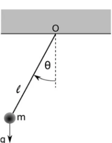
The K EPLER Problem
Introduction
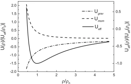
For this case, we schematically show in Fig.4.1 the effective potential (4.3) (solid black line), together with the gravitational potentialU./ (dashed-dotted line) and the centrifugal barrierUmom (dashed line). Here 0 is the distance from the minimum inUeff./.Ugrav./(dashed-dotted line) indicates the gravitational contribution while Umom./(dashed line) indicates the centrifugal barrier.
Numerical Treatment
4.4) is the integral representation of the ordinary differential equation (4.2), the approximation (4.16) corresponds to the approximation. Then an approximation method is called an explicit EULER method if it has the form It can be written as an approximation to Eq. 4.2) with the help of central differential drain DcnC1.
Ordinary Differential Equations: Initial Value Problems
Introduction
However, this is not actually a restriction since we can transform any n-order explicit differential equation into an associated set of first-order explicit differential equations. Therefore, we can relax the criterion discussed in point (i), that the differential equation must be distinct in y, to the criterion that the differential equation of order n must be distinct in the nth derivative of y, that is, y.n /. Although this equation appears to be simple, we must rely on numerical methods to obtain a solution.
Simple Integrators
Methods (1), (2) and (4) are also known as one-step methods, since only function values at times tn and tnC1 are used to propagate in time. In contrast, the leapfrog method is already a multi-step method since three different times appear in the expression.
T AYLOR Series Methods
R UNGE -K UTTA Methods
Our first choice is to replace ynC1=2 using the explicit EULER method, Eq. 5.24) is referred to as the explicit center rule. By analogy, we could have approximated synC1=2 using the resulting mean function value ynC1=2. Using RUNGE-KUTTA methods of the general form (5.32) one can develop methods of arbitrary precision.
Hamiltonian Systems: Symplectic Integrators
However, the discussion of such collocation methods [8] is far beyond the scope of this book. But you must always remember that there could be better methods to solve the problem. Remember, however, that the old workhorse's last ride may well lead you to the poor house: Bulirsch-Stoer or predictor-corrector methods may be much more efficient for problems where high accuracy is a requirement.
Symplectic E ULER
Symplectic R UNGE -K UTTA
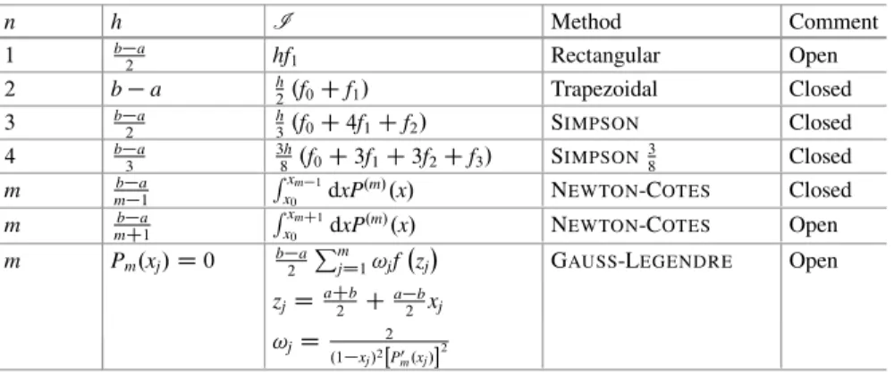
An Example: The K EPLER Problem, Revisited
Explicit E ULER
Implicit E ULER
The reason for this behavior is the methodological error in the method, which is accumulative and thus causes a violation of energy conservation. Thus, it is not surprising that the error in the implicit EULER method is also larger when H.t/ is determined. Crank, J., Nicolson, P.: A practical method for the numerical evaluation of solutions of partial differential equations of the heat conduction type.
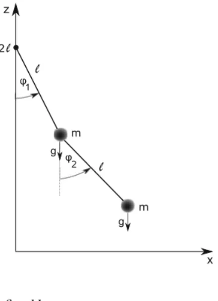
The Double Pendulum
H AMILTON ’s Equations
We find a description of the motion in phase space by the generalized momentapi,iD1; 2 axles.
Numerical Solution
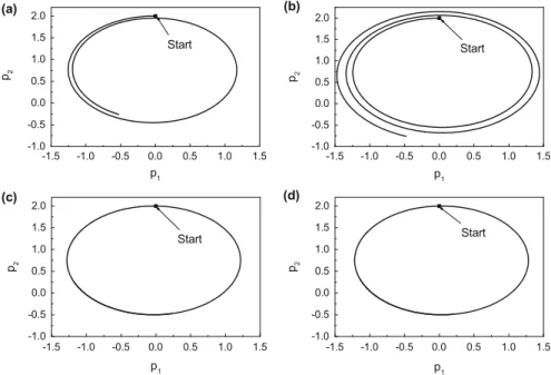
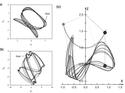
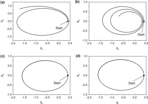
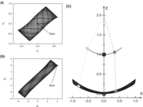
The dynamics depicted in Fig.6.4 are very similar to the one already discussed in Fig.6.2. The initial condition leading to the trajectory shown in Fig.6.5 differs only for mass 2 from the initial conditions leading to the trajectory in Fig.6.4. The situation shown in Fig.6.6 differs from the one of Fig.6.5 only by the initial condition for mass 2.
Numerical Analysis of Chaos
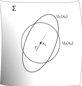
The idea was to reduce the investigation of the complete 2f-dimensional phase space trajectory x.t/ D 't.x0/ to the investigation of its intersections through a plane ˙transverse to the flow of the system. In this case the trajectory will not be periodic in general, and the next intersection'.x0/.x0/ ¤ x0. Whether or not one observes chaotic behavior depends on the choice of the initial conditions.
Molecular Dynamics
Introduction
Classical Molecular Dynamics
This method is called the STÖRMER-VERLET algorithm and serves as the initialization of a sequence of time steps. Furthermore, we note that Eq. 7.13) could also be obtained by using the central difference derivative to approximate the second time derivative in Eq. The STÖRMER-VERLET algorithm of Eq. 7.16) is time-reversible symmetric (invariant with respect to the transformation t ! t), i.e. reversible.
Numerical Implementation
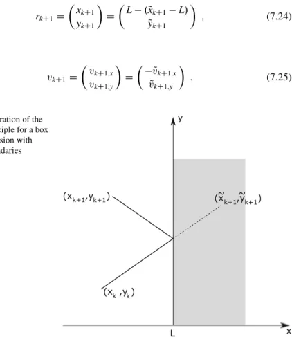
The choice of initial conditions greatly affects the time it takes for the system to reach thermal equilibrium. The top of the box is considered open (no periodic boundary condition or reflective boundary is imposed). Determine the momentum distribution (pi D mvi) of the particle and demonstrate that it follows a MAXWELL-BOLTZMAN distribution.
Numerics of Ordinary Differential Equations
Boundary Value Problems
Introduction
Finally, the boundary value problem (8.1) is referred to as inhomogeneous if the differential equation is homogeneous and the boundary conditions are also homogeneous. One of the most important types of boundary value problems in physics are second-order linear boundary value problems with discrete boundary conditions. In the following section, the finite difference method will be applied to solve boundary value problems of the form (8.4).
Finite Difference Approach
All these manipulations reduced the boundary value problem to a system of inhomogeneous linear equations, namely Eq. Although we have discussed the method of finite differences for the specific case of a second-order differential equation with decoupled boundary conditions, the same strategy can be used to derive similar methods for higher-order boundary value problems. Nevertheless, it was possible to reduce the boundary value problem to a system of linear equations that can be solved iteratively.
Shooting Methods
In addition, we note the following property of homogeneous boundary value problems: Suppose y.x/ is a solution of the boundary value problem (8.49), then every.x/Q Dy.x/ with D const will also be a solution of ( 8.49). This gives a very fast algorithm for solving the differential equation (8.54) with some initial values of the form (8.52). This was demonstrated on the example of a homogeneous boundary value problem of the one-dimensional stationary SCHRÖDINGER equation.
The One-Dimensional Stationary Heat Equation
Introduction
In the next section we apply the finite difference approximation to the boundary value problem (9.3) as discussed in section 8.2.
Finite Differences
Therefore, the finite difference approach to the boundary value problem (9.3) is exact and independent of the grid partition. This is not surprising since we already proved in Chapter 2 that finite difference derivatives are correct for linear functions.
A Second Scenario
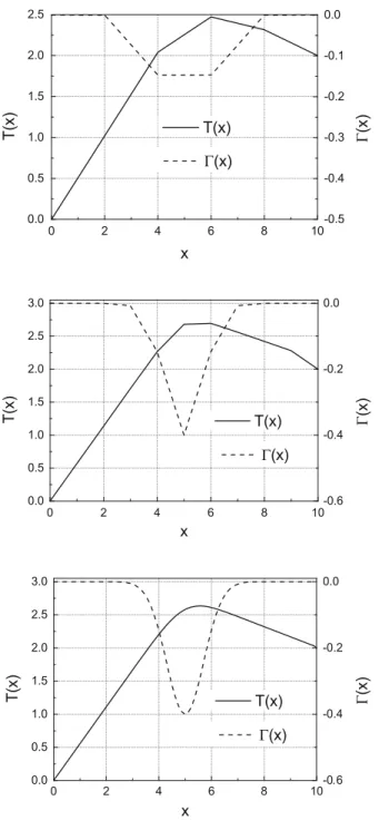
As the number of steps increases, we see, as expected, a refinement of the temperature profile. The methods of Section 8.2 were applied to find the numerical solution of the stationary heat equation with DIRICHLET boundary conditions. Investigate the three cases T0 > TN,T0 < TN, T0 D TN > 0, and study the influence of heat sink widtha on the temperature profile.
The One-Dimensional Stationary S CHRÖDINGER Equation
- Introduction
- A Simple Example: The Particle in a Box
- Numerical Solution
- Another Case
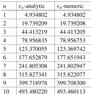
2m .x/CV.x/ .x/DE .x/ : (10.8) This equation will certainly not have solutions for arbitrary values of the energy E. In addition, Fig.10.1 shows the first five eigenvalues"n (right scale) as horizontal straight lines. In all cases, the eigenfunctions reflect the symmetry of the various potentialsv.s/Q, which becomes particularly transparent in Fig.10.3 for potentialtvQ1 .s/.
Partial Differential Equations
Introduction
This is of particular importance in the numerical treatment of hyperbolic PDEs, where the so-called COURANT-FRIEDRICHS-LEWY (CFL) condition determines the stability of the algorithm. Finally, we conclude this chapter with a discussion of the numerical solution of the time-dependent SCHRÖDINGER equation.
The P OISSON Equation
In detail, we want to solve the two-dimensional boundary value problem. where we absorbed0 in the charge density.x;y/. Note that a treatment of the three-dimensional case can be performed analogously. They only differ in the update procedure of the function values'it;swipe the grid points. Note that by using the iteration rule (11.12) the boundary conditions must be taken into account in an extra step.
The Time-Dependent Heat Equation
The time derivative in Eq. 11.17) can be approximated using methods already discussed in Chapter 5. In particular, one must decide whether the solution of Eq. 11.17) must be accessed by either an explicit or an implicit integrator. Figure 11.3 shows the time evolution of T.x;t/ at six different time steps as obtained with the explicit EULER method (11.19).
The Wave Equation
The function values for D 1 can be obtained from the initial conditions which must include a first-order time derivative of u.x;t/after Eq. 11.28) is a second-order differential equation with respect to time. ii). As in the case of parabolic problems, the explicit EULER approximation (11.30) will not be stable for arbitrary values of . Its importance stems from the fact that this condition is not limited to the wave equation, but applies to hyperbolic problems in general.

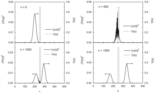
The Time-Dependent S CHRÖDINGER Equation
This problem can be solved by imposing the unitarity of the time evolution as an additional requirement. Calculate the electric field E.x;y/ using Eq. Calculate the time evolution of the temperature distribution T.x;t/ along a cylindrical rod described in Section 9.3. Calculate the time evolution of the square modulus of the wave functionj .x/j2 vsxfor a potentialV1.x/according to Eq.
Stochastic Methods
Pseudo-random Number Generators
Introduction
From a numerical point of view, all these applications have one common denominator: Random numbers are an essential tool, and so are random number generators. Therefore, a closer look at randomness in general and random number or sequence generation in particular is required. In addition, based on this discussion, we must formulate requirements for the random number generators to provide usable random numbers.
Different Methods
The seed is usually taken from, for example, the system time in order to avoid repetition in a sequence restart. To avoid using the same random number again, the ith element of the array is replaced by a new random number which, again, is calculated from (12.9) and (12.11). Again, the periodicity is highly dependent on the choice of parameters and the seed.
F IBONACCI Generators
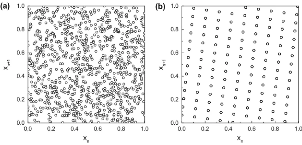
Quality Tests
Here we discuss some tests for checking whether a given finite sequence of numbers xn consists of uniformly distributed random numbers from the interval xn 2Œ0; 1.1. In box (a), the random numbers are nicely distributed within the unit square and show no obvious correlations. In Figure 12.2, we show three different histograms for N D 105, N D 106 and N D 107 uniformly distributed random numbers obtained with the PARK-MILLER linear congruential generator.