But the pressure of mathematics has certainly eased in recent times due to the strong (exponential) growth of numerical simulations. They can be skipped on first reading and display other illustrations of the chapter's topic.
The Foundations of Fluid Mechanics
A Short Historical Perspective
The Concept of a Fluid .1 Introduction.1Introduction
- Continuous Media
Fluid Kinematics
- The Concept of Fluid Particle
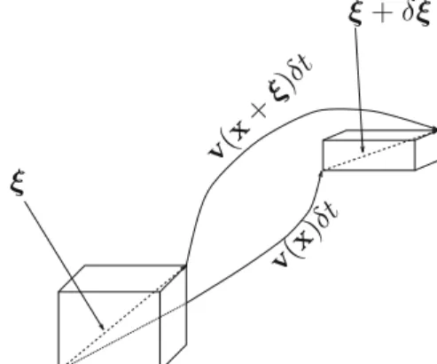
- The Lagrangian View
- The Eulerian View
- Material Derivatives
- Distortion of a Fluid Element
- Incompressible Fluids
- The Stream Function
- Evolution of an Integral Quantity Carried by the Fluid
The use of the velocity field as a function of position and time provides the Eulerian description of the flow. The term.vr/ is called the advection term and represents the transport of the quantity of the velocity field v.
The Laws of Fluid Motion
- Mass Conservation
- The Equation of Continuity
- Material Derivative with Mass Conservation
- Momentum Conservation
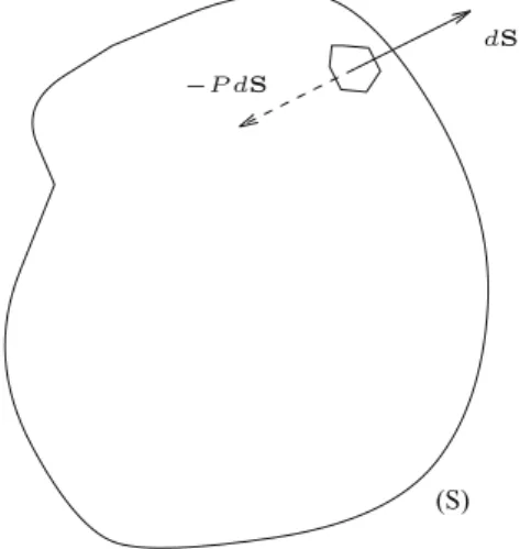
- The Stress Tensor Œ
- The Equation of Momentum
- Energy Conservation
- The Equation for Entropy
- The Constitutive Relations
3This implies in particular that the stress tensor is independent of the surface on which the stress is calculated. If we consider a fluid element, the above identity only says that the resultant of contact forces on a fluid particle is equal to the divergence of the stress tensor.
The Rheological Laws .1 The Pressure Stress
- The Perfect Fluid
- Newtonian Fluids
- The Viscosities
- The Microscopic Side
- The Momentum Equation and Navier–Stokes Equation
Such relationships are called the constitutive relationships and are specific to the microscopic nature of the fluid. This is a fairly small amount as the atmospheric pressure is of the order of 105 Pa.
The Thermal Behaviour
- The Heat Flux Surface Density
- The Equations of Internal Energy and Entropy
Expanding this expression and taking advantage of the fact that the trace of Œc is zero (Tr[c] = ıijcij=0), we find. This expression can be used to show that the Second Principle of Thermodynamics implies the positivity of transport coefficients such as viscosity and thermal conductivity.
Thermodynamics
- The Ideal Gas
- Liquids
- Barotropic Fluids
In; N, which expresses the internal energy as a function of various bulk quantities of the system (entropy, volume, number of particles, etc.). From this general relationship we derive the equations of state:. which defines the intensive quantities of the system, temperature T, pressure P or chemical potentialch.
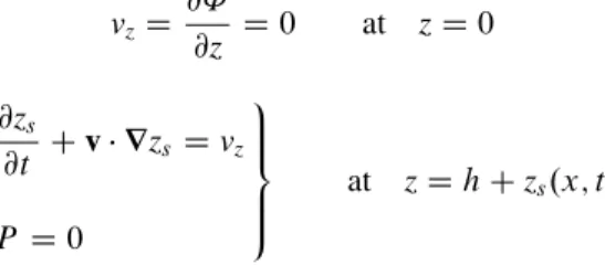
Boundary Conditions
- Boundary Conditions on the Velocity Field
- On a Solid Wall
- On a Free Surface
- The Stress-Free Boundary Conditions
- Boundary Conditions on Temperature
- Surface Tension
- Initial Conditions
In other words, on each side of the surface the voltage must be the same (up to the sign). Here n is the normal of the surface oriented from the liquid to the gas.
More About Rheological Laws: Non-Newtonian Fluids .1 The Limits of Newtonian Rheology
- The Non-Newtonian Rheological Laws
- Linear Viscoelasticity
- The Nonlinear Effects
- Extensional Viscosities
- The Solid–Fluid Transition
Such a behavior is understood as the result of the complexity of macromolecules that make up the liquid. For small values of the strain rate (T ! 1), we should recover the Newtonian fluid; hence from (1.78).
An Introduction to the Lagrangian Formalism
- The Equations of Motion
- The Eulerian and Lagrangian Variations
- Momentum Evolution
- An Example of the Use of the Lagrangian Formulation
One only needs to calculate the Jacobian of the transformation connecting the initial and final positions. Indeed, in this case, particles cannot cross and experience a constant gravitational force related to the mass remaining to the left and right of the particle.
Exercises
Further Reading
The Static of Fluids
- The Equations of Static
- Equilibrium in a Gravitational Field
- Pascal Theorem
- Atmospheres
- A Stratified Liquid Between Two Horizontal Plates
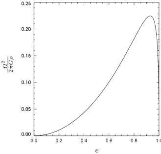
- Rotating Self-gravitating Fluids
- Some Properties of the Resultant Pressure Force
- Archimedes Theorem
- The Centre of Buoyancy
- The Total Pressure on a Wall
- Equilibria with Surface Tension
- Some Specific Figures of Equilibrium
- Equilibrium of Liquid Wetting a Solid
- Exercises
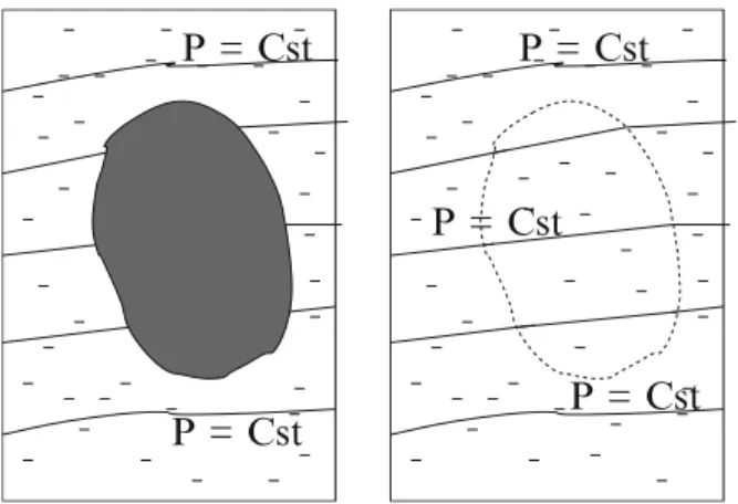
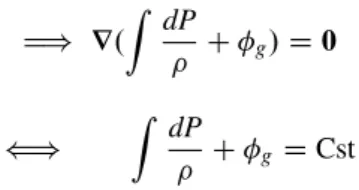
When we observe that the surface gravity of the sphere is g D GM=a2, we find the expression for", namely. When liquids are in equilibrium, one of the local body forces is the pressure gradient. What is the shape of the curve P .z /, the pressure as function of the height z (zD0 is the bottom of the container).
Assume that the envelope of the balloon is open in the lower part.
Flows of Perfect Fluids
Equations of Motions
- Other Forms of Euler’s Equation
Some Properties of Perfect Fluid Motions
- Bernoulli’s Theorem
- Statement and Proof
- The Pressure Field
- Two Examples Using Bernoulli’s Theorem
- Kelvin’s Theorem
- Statement
- Proof
- Interpretation
- Influence of Compressibility
This relation shows that the velocity at the foot of the waterfall is the velocity of a free particle falling from a height H. Kelvin's theorem (3.18) thus implies the constant of S12r water the constant of the angular momentum L of the liquid particle of massm. Kelvin's theorem shows that in the motion of an inviscid fluid, the angular momentum of the fluid particles is conserved.
We will see in Chapter 5 that P is simply the square of the local sound speed.
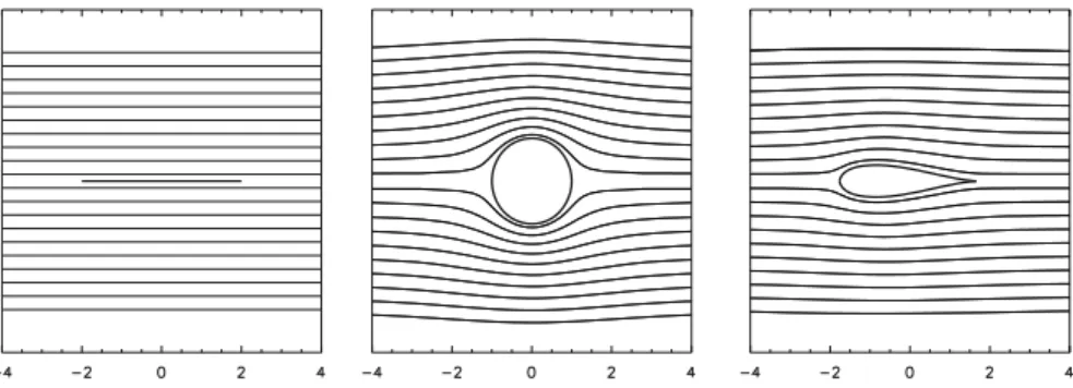
Irrotational Flows
- Definition and Basic Properties
- Role of Topology for an Irrotational Flow
- Lagrange’s Theorem
- Theorem of Minimum Kinetic Energy
- Electrostatic Analogy
- Plane Irrotational Flow of an Incompressible Fluid
- Equation for the Stream Function
- Inverse Analogy
- Forces Exerted by a Perfect Fluid
- d’Alembert’s Paradox
- Case Where the Obstacle is Accelerated
- Drag and Lift of Two-Dimensional Flows
The uniqueness (up to within an additive constant) of the solution follows from Laplace's equation which is satisfied by the potential˚. The second boundary condition arises from the properties of the solutions of Laplace's equation (see the mathematical supplement). The force applied to the solid is still the result of the compressive forces, that is.
This integral is equal to zero because of the boundary conditions on the solid body and because of the shape of the velocity at infinity.
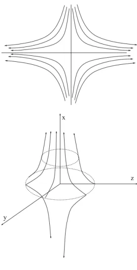
Flows with Vorticity
- The Dynamics of Vorticity
- Flow Generated by a Distribution of Vorticity: Analogy with Magnetismwith Magnetism
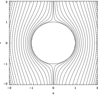
- Examples of Vortex Flows
- Vortex Sheets
- Hill’s Vortex
- The Vortex Ring
It is then easy to find the distribution of the associated velocity; is sufficient. The velocity field on the outside of the core was chosen so that the velocity is continuous atrDa. The two constants A and Bar are such that the velocity is right at the center of the sphere (so that BD0) and that the radial velocity vanishes at trDa.
This velocity represents the speed of the vortex relative to the fluid at infinity; it is uniform and along the vortex axis.
Problems
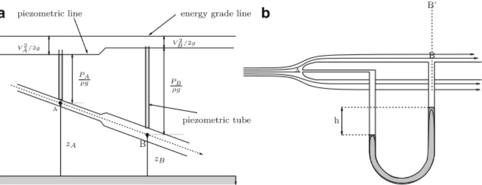
One now adds to the reservoir a horizontal pipe of length `, and of very small diameter compared to that of the tank. The pressure of the city water service is 6 bar; if the length of the connecting pipe from the main pipe to the basin is 10 m, what is the elapsed time when you open the tap. We are interested in the small oscillations of the liquid height over the mean value h0; these oscillations occur, for example, when the tube is slightly shaken.
Neglecting airflow, express the pressure in the bubble in terms of the radius.
Appendix: Flow Past a Plane at Incidence
The points z z0 on the flat plate correspond to zbeing on the circle, i.e. zDRei,2Œ0; 2. Note that the flow at the leading edge is also singular, but this singularity can be eliminated by rounding the profile as shown in Figure 3.4c. Regarding vorticity dynamics, further development of the remarks presented here will be found in the dynamics of SaffmanVortex (1992) or in eddy currents of Ting and KleinViscous (1991).
As for the properties of the Euler equation, extended material is proposed in Zeytounian Mécanique des fluides fundamentale (1991).
Flows of Incompressible Viscous Fluids
Some General Properties .1 The Equations of Motion.1The Equations of Motion
- Law of Similarity
- Discussion
This non-dimensional number is the only parameter that interferes with the equations of motion of an incompressible viscous fluid. A practical application of the similarity relation is the use of reduced models to study some complex flows. System (4.7) gives us the first example of flow equations written with nondimensional variables.
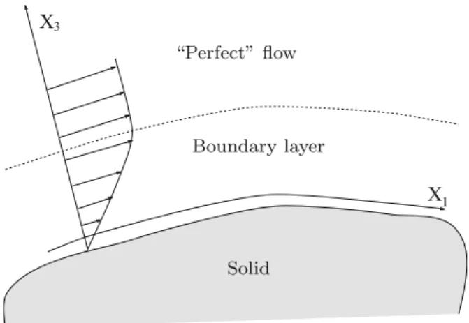
This singularity is at the origin of boundary layers, which appear when the Reynolds number is very large (see Section 4.3).
Creeping Flows
- Stokes’ Equation
- Variational Principle
- Flow Around a Sphere
- Oseen’s Equation
- The Lubrication Layer
Another important consequence of the linearity of the Stokes equation is the uniqueness of the solution for a given set of boundary conditions. This means that the solutions (4.10) make the extrema a functional of the velocity field defined on the space occupied by the fluid. For this we note that the dissipation is a linear function of the square of the velocity gradient.
This result shows that the pressure increases strongly when the thickness of the liquid layer disappears.
Boundary Layer Theory
- Perfect Fluids and Viscous Fluids
- Method of Resolution
- Flow Outside the Boundary Layer
- Flow Inside the Boundary Layer
- Separation of the Boundary Layer
- Example of the Laminar Boundary Layer: Blasius’
In the boundary layer viscosity is important and the full equation must be solved. The thickness of the boundary layer, and hence the extended coordinate, is such that@@QfzQ D O.1/; that is, the normal variations of the boundary layer functions, respectively. This last expression shows that the boundary layer equations are nonlinear and third order.
The value ofuQ1;z thus plays the role of the boundary value for the first-order terms in the perfect domain.
Some Classic Examples
- Poiseuille’s Flow
- Stationary Regime
- Transients to a Poiseuille’s Flow
- Head Loss in a Pipe
- Regular Head Losses
- Singular Head Losses
- Flows Around Solids
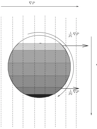
It thickens as the square root of the distance to the entrance as illustrated in Fig.4.5. We have examined here the case of a sudden enlargement of the cross-section; in the opposite case of a cross-section that suddenly narrows, there is also some head loss, but not as great. When the Reynolds number is small compared to unity, vorticity fills the entire space, although it decreases like1=r2 as shown by (4.19) in the case of the sphere.
Here we see that this symmetry breaking actually occurs through the rise of the wake on the downstream side.
Forces Exerted on a Solid
- General Expression of the Total Force
- Coefficient of Drag and Lift
- Example: Stokes’ Force
The expression for the force acting on a rigid body is seldom obtainable by direct calculation, especially when the Reynolds number is large compared to unity. When the Reynolds number is large, the pressure field due to fluid inertia is the main source of stresses acting on a solid moving in a fluid. To conclude this section, we consider the case of a uniform motion of a sphere in a viscous fluid when the Reynolds number is very small.
The solution we obtained in Section 4.2.3 allows us to calculate the expression of the resultant force.
Exercises
We take the Prandtl equations of the laminar boundary layer (4.37), but look for solutions more general than those of Blasius. We put Q0;x D U.x/f ./anduQ1;z D V .x/g./, where is still the self-similarity variable and U.x/thex-component of the velocity at infinity. a) Give the expression for @p0=@x as a function for U.x/. b) Show that the existence of such solutions means that U.x/; In .x/inb.x/. c) Derive the general form of U.x/inb.x/. d) Show that if we choosesc1=2Cc2D1 (why is this always possible?), then F DR. where is the constant associated with c1; c2; c3. e). The material of this chapter belongs to the very foundation of fluid mechanics and can therefore be found in all introductory fluid mechanics books; for example, Batchelor (1967), Faber (1995), Guyon et al.
Waves in Fluids
Ideas on Disturbances
- Equation of a Disturbance
- Analysis of an Infinitesimal Disturbance
- Local Analysis
- Global Analysis
- Disturbances with Finite Amplitude
- Waves and Instabilities
Local analysis is simpler because the shape of the disturbances is known in advance. When the boundary conditions or heterogeneities of the perturbed system cannot be neglected, the plane waveform cannot be imposed on the perturbations. Simultaneously, we determine the associated eigenvalues which give the point spectrum (set of eigenvalues) of the operator L.
When the amplitude of the disturbances cannot be neglected, the problem becomes very complicated due to the non-linearities of the equations.
Sound
- Equation of Propagation
- The Dispersion Relation
- Examples of Acoustic Modes in Wind Instruments
- The Flute
- The Clarinet
Let's calculate the order of magnitude of the speed of sound in air at 300 K. The speed of sound is of the same order of magnitude as the effective speed of 2 gas molecules. Let us now consider the orientation of the velocity field associated with the wave and the wave vector.
At the extreme parts of the tube, the pressure is fixed (that is atmospheric pressure), so the pressure disturbance disappears there.3 These two boundary conditions allow us to write.
Surface Waves
- Surface Gravity Waves
- In Deep Water
- In Shallow Water
- Capillary Waves
To be more precise, we consider the case of an interface between air and water and deal with the motion of the two fluids at the same time. If we now assume that the amplitudes of movements are small, we find from (1.63) that. These two relations show that the waves are dispersive: the long-wavelength waves are the fastest.
If the depth of the water is not infinite (and especially if it is smaller than the wavelength of the waves), the dispersion relation is greatly simplified.
Internal Gravity Waves
For such waves, the restoring force is the driving force which has a preferred (vertical) direction. To become more familiar with these waves, we consider the following idealized situation: a quasi-incompressible fluid (such as water) is in equilibrium under the effect of gravity. We further assume that the variations of density associated with the variations of temperature are negligible, except for those that generate the driving force (this is the Boussinesq approximation that we will thoroughly describe in Chapter 7).
We combine this equation with !ıvzDikzp=X˛ıT0gandi !ıT0Cˇıv0zD0 to finally obtain the following dispersion relation:.
Waves Associated with Discontinuities
- Propagation of a Disturbance as a Function of the Mach NumberNumber
- Equations for a Finite-Amplitude Sound Wave
- The Equations of Characteristics
- Example: The Compression Wave
- Interface and Jump Conditions
- Relations Between Upstream and Downstream Quantities in an Orthogonal Shockin an Orthogonal Shock
- Strong and Weak Shocks
- Radiative Shocks
- The Hydraulic Jump
For example, the mass flow must be the same on each side of the stroke. They can be used to overwrite downstream quantities (index 2) as a function of upstream quantities. These relationships allow us to determine the state of the liquid after the passage of the shock wave.
Let us now show that the entropy jump is an increasing function of the Mach number.
Solitary Waves
- The Korteweg and de Vries Equation
- The Solitary Wave
- Elementary Analysis of the KdV Equation
We also note that the horizontal scale of the wave (the width of the "bump") is given by. The properties of the KdV equation are numerous and we could write a whole book on it. Here, we indulge in an elementary analysis to assess the role of the various terms involved in this equation.
We can now take a look at how this term contributes to the propagation of the wave packet.