Physical processes leading to export of ﬁxed carbon out of the surface ocean

(1)

Doctor of Philosophy

CALIFORNIA INSTITUTE OF TECHNOLOGY Pasadena, California

2019

Defended 29 May 2019

(2)

(3)

(4)

ACKNOWLEDGEMENTS

Thanks to Kim and Kevin Erickson, my parents, for supporting me at all stages of my life’s journey, believing in me at every step of the way, and encouraging me to pursue opportunities that would help me grow;

To Andy Thompson, my Ph.D. advisor, for his excitement and passion for science, his unwavering support of my development as a scientist throughout the past six years, his encouragement of my taking on research projects not directly related to my thesis, his willingness to take on projects that stretched his own area of expertise, his thoughtful advice on a variety of topics throughout my graduate school tenure, and for always treating me as a scientific collaborator;

To Giuliana Viglione, for being a constant sounding board, for helping me tell more cohesive and coherent stories, and for always encouraging me to expand my boundaries;

To Xiaozhou Ruan, for always being willing to help me through fluid dynamics problems and for being a constant supportive presence throughout our time in the Thompson group;

To the entire Thompson group at Caltech, past and present, for a welcoming and invigorating research atmosphere;

To Jess Adkins, for chairing my thesis advisory committee and for first introducing me to oceanography, and especially for showing me how exciting and interconnected all of the different sciences are when applied to the oceans;

To Christian Frankenberg, for being a member of my thesis advisory committee and for spending so much time helping me understand remote sensing and inverse modeling;

To Michelle Gierach, for being a member of my thesis advisory committee and inviting me up to JPL on numerous occasions to give seminars or to talk about ongoing research projects;

To Nicolas Cassar, for helping me to understand biological oceanography concepts and feel like I could make a contribution to the field;

To Kevin Arrigo, for taking me on my first research cruise and treating me like an independent scientist from the very beginning;

(5)

enthusiasm about science has helped me throughout; and

To Hannah Joy-Warren, Ivona Cetinić, Anna Ho, Hall Daily, Dave Siegel, and the many other people who gave me encouragement along the way.

(6)

ABSTRACT

The ocean sequesters carbon on long time scales by depositing it deep in the ocean, where it is no longer in contact with the atmosphere. This sequestration is also termed

“carbon export”, and is accomplished via a vertical flux of carbon into the interior of the ocean. Marine photosynthesis by phytoplankton, which consume carbon dioxide dissolved in the surface ocean and are transported to depth to be eventually remineralized or form sediments at the ocean surface, is a key component of this flux (the biological pump). This mechanism is primarily thought to occur via sinking of particulates. However, research over the past few decades has highlighted the role of instabilities at the “submesoscale”, or 0.1–20 km, to induce large,O(100 m day⁻¹) vertical velocities in the ocean. These vertical velocities can potentially subduct carbon from the surface ocean into the interior, where it would contribute to export.

Observations of the ocean are, however, rarely made at scales which would detect these submesoscale instabilities. In this thesis, I use in situ observations from autonomous underwater vehicles, Seagliders, which make measurements in the upper 1000 m of the water column at horizontal scales of 1–3 km, to understand when and where submesoscale instabilities are present, and the extent to which they act to transport biologically fixed carbon out of the surface ocean. Three different types of instabilities are active in the surface mixed layer: baroclinic, gravitational, and symmetric. Each of these has potential to subduct material below the mixed layer; however, these instabilities are generally strongest during the winter, when biological production is at its minimum. An interesting exception is in southern Drake Passage, where interactions between the intense frontal system and the continental shelf result in subduction of water masses off the continental shelf during summer, when phytoplankton are photosynthesizing. In general, however, carbon export via submesoscale instabilities is expected to be largest during spring, when phytoplankton become more productive but conditions can still be ripe for submesoscale subduction. Scaling up these observations to the global ocean system is difficult because in situ observations at submesoscales are sparse. This thesis explores the ability of surface flux measurements, from reanalysis products and remote sensing measurements, to accurately depict carbon export via subduction processes by modeling the water profile in a one-dimensional model following Lagrangian floats in the ocean. This approach holds promise to advance the ultimate goal of determining the global effect of submesoscale-driven carbon export.

(7)

Erickson, ZK, C Frankenberg, DR Thompson, AF Thompson, and M Gierach (2019).

“Remote Sensing of Chlorophyll Fluorescence in the Ocean Using Imaging Spec- trometry: Toward a Vertical Profile of Fluorescence”. In:Geophysical Research Letters46.3, pp. 1571–1579. doi:10.1029/2018GL081273.

Z.K.E. assisted in writing the proposal for this research, analyzed the data, and wrote the manuscript.

Erickson, ZK and AF Thompson (2018). “The seasonality of physically driven export at submesoscales in the Northeast Atlantic Ocean”. In: Global Biogeochemical Cycles32.8, pp. 1144–1162. doi:10.1029/2018GB005927.

Z.K.E. conceived the project, analyzed the data, and wrote the manuscript.

Arrigo, KR et al. (2017). “Early spring phytoplankton dynamics in the Western Antarctic Peninsula”. In: Journal of Geophysical Research: Oceans 122.12, pp. 9350–9369. doi:10.1002/2017JC013281.

Z.K.E. assisted in the collection of the data, processed the CTD data, calibrated the salinity and oxygen measurements, analyzed the ADCP data, wrote Section 3.2 (Hydrography), and made Figures 1,4–6.

Thompson, AF et al. (2017). “Satellites to seafloor: Toward fully autonomous ocean sampling”. In: Oceanography 30.2, pp. 160–168. doi: 10 . 5670 / oceanog . 2017.238.

Z.K.E. assisted in the collection of the data and the analysis of the data.

Erickson, ZK, AF Thompson, N Cassar, J Sprintall, and MR Mazloff (2016). “An advective mechanism for deep chlorophyll maxima formation in southern Drake Passage”. In:Geophysical Research Letters 43.20, pp. 10–846. doi: 10.1002/

2016GL070565.

Z.K.E. conceived the paper idea, analyzed the data, and wrote the manuscript.

(8)

LIST OF ILLUSTRATIONS

Number Page

2.1 Overview of OSMOSIS region and measurement locations. . . 16 2.2 Mixed layer depths and seasonal density and vertical buoyancy strat-

ification profiles. . . 19 2.3 Spice transects from glider measurements and model output. . . 20 2.4 Model snapshots of spice along isopycnal surfaces. . . 21 2.5 Frequency spectra of kinetic energy, potential energy, and spice vari-

ance from model output and mooring data. . . 22 2.6 Structure functions for kinetic energy, potential energy, and spice

from model output, mooring data, and glider data at a single depth. . 24 2.7 Example of a fit to a power-law curve for structure function results. . 25 2.8 Best-fit slopes of power-law curves for kinetic energy, potential en-

ergy, and spice structure functions. . . 26 2.9 Best-fit offset of power-law curves for kinetic energy, potential energy,

and spice structure functions. . . 28 2.10 Best-fit offsets of kinetic energy and potential energy applied to mov-

ing 30-day windows at 50 and 350 m for model output, mooring data, and glider data. . . 29 2.11 Uncertainty in glider position as a function of depth. . . 35 2.12 Histogram of separation distances in glider pairings at 200 m depth. . 36 3.1 Overview of OSMOSIS location and glider measurements. . . 41 3.2 Average surface chlorophyll concentrations from MODIS Aqua ob-

servations and fromin situglider data. . . 45 3.3 Calibration of glider chlorophyll data to satellite estimates. . . 48 3.4 Scatterplot of coincident backscatter measurements at 470 and 700 nm. 49 3.5 Chlorophyll and backscatter fromin situglider measurements. . . 50 3.6 Community index fromin situglider measurements. . . 52 3.7 Potential vorticity and apparent oxygen utilization fromin situglider

measurements. . . 53 3.8 Potential vorticity and apparent oxygen utilization fromin situglider

measurements along potential density surfaces. . . 55

(11)

3.13 Schematic showing the seasonal cycles of mixed layer depth, strength of the pycnocline, vertical motions associated with submesoscale instabilities, particulate organic carbon concentrations, and carbon export. . . 62 4.1 Overview of the ChinStrAP study region and measurements. . . 68 4.2 Winter water capping and development of an along-isopycnal poten-

tial vorticity gradient. . . 72 4.3 Schematic of mechanism generating off-shelf deep chlorophyll maxima. 73 4.4 Layer-wise horizontal velocities from the Southern Ocean model. . . 75 5.1 PWP model processes. . . 83 5.2 Submesoscale processes incorporated into the PWP model. . . 84 5.3 PWP model run with a simple seasonal cycle without submesoscale

dynamics. . . 87 5.4 PWP model run with a simple seasonal cycle with additional subme-

soscale dynamics. . . 88 5.5 Locations of Argo floats. . . 90 5.6 Surface forcings used in the PWP model. . . 91 5.7 Horizontal buoyancy gradient observations from OSMOSIS gliders

compared with that derived from MODIS Aqua sea surface temperature gradients. . . 92 5.8 Mixed layer depths for Argo floats using in situ measurements and

PWP model results. . . 93 5.9 Temperature for Argo floats using in situ measurements and PWP

model results. . . 93 5.10 Sensible and latent heat in the PWP model compared with NCEP

reanalysis values. . . 94

(12)

5.11 Surface carbon concentrations for Argo floats usingin situdata and PWP model results. . . 95 5.12 Carbon export calculated using the PWP model. . . 96 5.13 Ratio between vertical derivatives of temperature in the mixed layer

following baroclinic mixed layer instability and in the pycnocline, and the ratio of export estimates using different parameterizations. . . 98

(13)

(14)

C h a p t e r 1

INTRODUCTION

1.1 Motivation

The ocean plays a major role in the global carbon cycle (Field et al., 1998). As the largest reservoir of carbon in the Earth system (besides the solid earth), air-sea gas transfer plays a key role in modulating the atmospheric carbon dioxide content over geologic time (Sarmiento and Toggweiler, 1984). On shorter, yearly and decadal timescales, the ocean acts to absorb roughly one quarter of anthropogenic carbon dioxide emissions, limiting the rise of carbon dioxide in the atmosphere (le Quéré et al., 2018).

This absorption of carbon dioxide is strongly time- and region-dependent, and pro- ceeds by a variety of mechanisms. The total uptake of carbon dioxide is dominated by gas transfer across the air-sea interface into the surface ocean (a small amount is also present from river inflow), estimated at 80 Pg C/yr, or roughly ten-fold greater then the total anthropogenic emissions. However, most of this carbon (estimated at 78 Pg C/yr) is ultimately fluxed back through the air-sea interface, and the net build-up within the ocean is small, on the order of 2 Pg C/yr (IPCC, 2013).

This small build-up of carbon in the oceans is a consequence of longer-term carbon sequestration, which occurs when carbon is vertically advected out of the surface mixed layer of the ocean, which is in contact with the atmosphere. The vertical flux of carbon is related to either the sinking speed of particulate organic carbon or to vertical subduction of water masses containing fixed carbon. This thesis is primarily concerned with the second term, and especially the impact of submesoscale instabilities on the subduction of water masses out of the surface ocean.

1.2 Introduction to submesoscales

At scales ofO(100−1000 km)the ocean is approximately in geostrophic balance, meaning horizontal pressure gradients are balanced by the Coriolis force, vertical shear in the horizontal flow is small, and vertical motions are negligible. Geostrophy is characterized by small Rossby numbers Ro = ^U_{f L}, whereU,L are characteristic velocity and length scales and f is the planetary vorticity, and large Richardson numbersRi= _U^N2²

z, whereN²= bz is the vertical buoyancy frequency and subscripts

(15)

Vertical motion at submesoscales occurs via instabilities that are generally caused by surface forcing. We return to these in a later chapter, but at the moment it is useful to define a crucial variable in the ocean: potential vorticity (PV), defined as

PV = (f +∇ ×u) · ∇b, (1.1) where∇is the full three-dimensional gradient operator andbis the buoyancy. (We also make the “traditional approximation” the planetary vorticity only exists along the vertical axis.) Decomposing,

PV = bx(w_y−vz)+b_y(uz−wx)+bz(f +vx −u_y). (1.2) A common approximation is to assume that gradients associated with the vertical velocityware small. If we also assume the ocean is in geostrophic and hydrostatic balance,

uz,vz = bx

f ,−b_y

f , (1.3)

and

PV = f N²+ζN²− f⁻¹M⁴, (1.4) where M² = ∇_hb. We assume in the following (short) discussion that f > 0 (true for the northern hemisphere); in the southern hemisphere f < 0 and some signs change, but the same qualitative observations hold. In a non-convecting ocean where N² > 0, the first term always contributes to positive PV, the third term is always negative, and the second term varies depending on the sign of ζ. Here positive PV is stabilizing and negative PV destabilizing, so horizontal buoyancy gradients (M²) are always destabilizing. We can substitute (1.3) into our previous equation for Ri to obtain a so-called "balanced" Richardson number

Rib= f²N²

M⁴ . (1.5)

(16)

Then, usingRo= ^ζ_f, our PV equation becomes

PV = f N²(1+Ro−Ri⁻_b¹), (1.6) and we see that large negative (or at least order-unity) Rossby and small (or at least order-unity) Richardson numbers lead to negative, or destabilizing, PV.

1.3 Carbon export

This thesis is focused on understanding how biologically-generated marine carbon is sequestered in the ocean beneath the surface ocean layers. For the purpose of this thesis, this quantity will be defined as “carbon export” (Passow and Carlson, 2012). However, the term “export” is nebulous without a clear associated timescale.

For example, carbon which is subducted below the mixed layer during summer may be re-entrained as the mixed layer deepens in winter. Therefore, many studies, including Chapter 3 in this thesis, focus on export during the winter and spring months. Another complication is that in up-welling favorable regions biological carbon may also be remineralized at depth and then transported to the surface, where the carbon dioxide out-gasses into the atmosphere; this thesis does not address this issue except in a one-dimensional sense in Chapter 6.

A useful metric of export is thee-ratio, which is the ratio between primary production within the surface euphotic layer, bounded by zeu, and the amount of fixed carbon which descends below the zeu. For convenience, a fixed depth, such as 100 m, is sometimes taken for zeu. Deeper than this depth, fixed carbon is subject to remineralization but not growth. In a landmark study, J. Martin et al. (1987) used conical traps at different depths at nine stations in the northeast Pacific ocean to calculate a best-fit remineralization curve,

F(z)= F₁₀₀ z

100 −b

, (1.7)

whereFis the flux at depth z, F₁₀₀is the flux atzeu=100 m, and the exponentbis fit to available data. They found a remarkably constant fit forb = 0.86, suggesting that remineralization rates were roughly constant in the ocean. In a later study, (Berelson, 2001) challenged this idea, findingbfrom 0.6 to 1.3. The concept of an exponential power law is largely empirical, and some evidence has suggested more complex forms, such as including two power laws for labile and ballast material (Armstrong et al., 2001).

What processes control the e-ratio and Martin’s b exponent? Simple food-web models typically decompose biomass into phytoplankton, zooplankton, and detritus.

(17)

backscatter, nitrate, phosphate, oxygen, and solar radiation can be used. Generally, these measurements must be made in a Lagrangian sense, meaning following a parcel of water (rather than at a single latitude/longitude location) over a period of days to months. In one observational study in the west Antactic Peninsula region, Stukel et al. (2015) calculated net production based on nitrate uptake in incubation exper- iments from water samples, net nitrate drawdown in the water column, and oxygen production (relative to argon, a gas that has similar air-sea transfer coefficients), and found good agreement between each of these three methodologies. However, their estimates of net carbon flux, from sediment traps and thorium isotopes, were significantly lower than the net estimated production, suggesting that other processes, such as diapycnal diffusion of nitrate and transport of particles across the base of the mixed layer, also had a substantial effect. In another example, (Alkire et al., 2012) used data collected from the North Atlantic during the spring bloom to compute net community production within the surface ocean using changes in nitrate, oxygen, and particulate organic carbon (POC) concentrations. They tracked an entire spring bloom cycle from initiation to termination, and found that export was highest during the time period of the main bloom. In this thesis we return to this issue of Lagrangian bloom measurements in Chapter 5, where we use a simple model to estimate export using only surface properties.

Export on larger scales can be estimated via surface measurements, which typically combine a productivity model (e.g. Eppley et al. (1985), Morel and Berthon (1989), Behrenfeld and Falkowski (1997), and Behrenfeld et al. (2005)) with an estimate of the e-ratio. Laws et al. (2000) uses a simple food web model to show a strong dependence onewith total net primary production and temperature, with the highest values for highly productive ecosystems and cold temperatures — the former is

(18)

characterized by large, quickly-growing and fast-sinking particles, and the latter is due to lower respiration rates at colder temperatures. Separating phytoplankton into two size classes (i.e. fast-growing, fast-sinking and slow-growing, neutrally- buoyant) was found to increase the skill of an empirical model at predicting e at different global sites (Dunne et al., 2005; Siegel et al., 2014). The dominance of these fast-growing size classes in high latitudes leads to an increase in e in polar regions (Henson et al., 2012).

However, the bexponent also varies greatly, including with latitude. Specifically, large, fast-growing, polar phytoplankton tend to be highly labile with respect to the more refractory slow-growing phytoplankton in low latitudes, causing their vertical transmission to be low (e.g., large b value) (Henson et al., 2012). Importantly, these characteristics of a phytoplankton bloom can change temporally as well as spatially. Buesseler and Boyd (2009) showed that from spring to summer many phytoplankton blooms evolve to have less export but higher transmission within the ocean interior as a result of a temporal shift in ecosystem composition (see also Siegel et al. (2016)).

1.4 Marine biology observations from Seagliders

Seagliders (or, “gliders”) are autonomous underwater vehicles that can be deployed for months at a time, making them an attractive and (comparatively) cheap alternative to traditional ship-based ocean measurements (Rudnick, 2016). They are buoyancy- driven vehicles that can travel at a horizontal speed of about 1 km hour⁻¹ and complete a dive to their maximum rated depth of 1000 m in about 5 hours.

Typical physical measurements include temperature, salinity, pressure, and oxygen concentration. In this thesis we also use biological measurements of chlorophyll fluorescence and backscatter, which give information on chlorophyll and particulate organic carbon (POC) concentrations, respectively.

Chlorophyll fluorescence

Chlorophyll molecules fluorescence when exposed to sunlight (Kautsky and Hirsch, 1931), and measurements of chlorophyll fluorescence give information on chlorophyll concentration and organism physiology (e.g., whether or not the organism is nutrient stressed). Fluorescence measurements are made by exciting the water column with light in a specific wavelength range, and then measuring emitted light (fluorescence) at a different wavelength. The chlorophyll fluoremeter used in this thesis has an excitation wavelength of 470 nm and a retrieved fluorescence

(19)

under high light regimes where photosynthesis is not limited by photon availability, a variety of mechanisms exist to “quench”, or use up, radiation. These are collectively known as non-photochemical quenching (NPQ) processes, and typically act to draw down chlorophyll fluorescence in the upper part of the water column.

The most common method to deal with NPQ is to disregard any fluorescence measurements made during the daytime or, if there is information on PAR, above a certain PAR threshold. This is the method used in Chapter 3. However, often disregarding all daytime measurements too drastically limits the amount of useful data. A variety of schemes have been developed to correct for NPQ effects. If the mixed layers are deeper than the effects of NPQ (determined by whether or not the profile of fluorescence starts to decrease within the mixed layer), one method is simply to extrapolate the maximum fluorescence within the mixed layer to the surface. However, this obviously is not an ideal solution, as it prohibits knowledge of any type of chlorophyll increase within the mixed layer, which may be present if the mixed layer is substantially different from the layer of active mixing (Brainerd and Gregg, 1995; Taylor and Ferrari, 2011; Ferrari et al., 2015). This method also does not effectively correct for NPQ effects if these extend throughout the mixed layer. Another alternative is to rely on other measurements. For example, if backscattering measurements were also made, they can be used as a proxy for fluorescence during the day by being scaled with the average nighttime mixed layer backscatter:fluorescence ratio. This is the method used in Chapter 4. In these above examples, fluorescence data are simply discarded (and replaced with some other source of information) when they are determined to be affected by NPQ.

Alternatively, one can attempt to model the effect of NPQ on fluorescence and come up with a scaling factor based on PAR. This was done, for example, in a recent study by Xing et al. (2018), where they assumed a sigmoidal effect of NPQ with respect

(20)

to PAR.

Backscatter

Another biological measurement available on autonomous underwater vehicles such as Seagliders is backscatter, which measures the amount of emitted light scattered back to the sensor at a given wavelength by the seawater. Backscattering is strongly dependent on particle size and composition, but has been found to be linearly proportional to phytoplankton concentrations and, more generally, to particulate organic carbon (POC) in the ocean (Baker et al., 2001; Stramski et al., 2008; Boss et al., 2008). Analyses that seek to determine actual concentrations of phytoplankton or POC require additional, and labor-intensive, particle-counting measurements to find these region-specific parameters. These are typically not possible for Seaglider de- ployents, and accordingly in this thesis (Chapters 3 and 4) we simply use backscatter as a measurement which is understood to be proportional to POC.

1.5 Impact

This thesis focuses on the role of submesoscale instabilities in subducting carbon out of the surface ocean and into the interior, thus contributing to carbon export. In the open ocean there is likely a small window of time, particularly during spring, where this effect may contribute significantly to carbon export. Most of the results in this thesis are based on data from Seagliders, and accordingly do not have the ability to constrain fluxes to the degree that ship-based measurements involving water sampling would allow. However, within the time span during which this thesis was prepared, three major initiatives have begun that should allow the effect of submesoscale dynamics on carbon export to be much better quantified: EXPORTS (EXport Processes in Ocean from RemoTe Sensing) in the Pacific and Atlantic Oceans, S-MODE (Sub-Mesoscale Ocean Dynamics Experiment) in the California Current System, and Bio-Argo. This last project is an ongoing observational cam- paign that was initiated near the start of this thesis, and data from which was used in the last chapter. The goal of at least one of these campaigns, EXPORTS, is to quantify carbon export from surface measurements, which aligns very closely to the goals of this thesis, and especially the last chapter, which aims to quantify carbon export following a Lagrangian parcel (as will be done in EXPORTS).

The observational results presented in this thesis come from two very different areas.

Carbon export via submesoscale subduction in the open Atlantic ocean, presented in Chapter 3, is limited due to the low temporal overlap between large submesoscale

(21)

heating, and is contemporaneous with a phytoplankton bloom, leading for a much higher potential for total carbon export. However, it is unclear to what extent these dynamics prevail in other regions of the ocean.

The ultimate goal of this thesis is to both mechanistically determine which submesoscale instabilities lead to carbon export, and understand how important they are in contributing to total export. This dissertation can be compared to a recent study by Omand et al. (2015), which estimated carbon export due to submesoscale baroclinic mixed layer instability (BMLI). This study concluded that springtime carbon export caused by this single instability could in certain regions of the ocean contribute nearly half of all carbon export. However, this prediction was a result of a simplified version of BMLI which does not accurately portray the vertical profile of subduction. In Chapter 5 of this thesis, we apply BMLI to a simple, 1-D model of the ocean, and show that it can in fact contribute much more to carbon export than predicted by Omand et al. (2015). We also analytically show that the prediction given by Omand et al. (2015) is generally accurate under conditions of strong BMLI, but that the simplified prediction can be up to four times too small under conditions of weaker BMLI, indicating that regions with low predicted submesoscale-induced carbon export may be under-estimated.

However, this thesis also points to other submesoscale instabilities, particularly symmetric (Chapter 3) and wind-driven gravitational (Chapter 5) as also contributing substantially to carbon export through subducting fixed carbon below the mixed layer and deepening the mixed layer leading to an increase in carbon export following restratification, respectively. While there are major limitations to including a representation of symmetric instability in a 1-D, surface-forced model such as is developed in Chapter 5, this model does permit understanding the spatial and

(22)

temporal signatures of both BMLI and wind-driven gravitational instabilities. In this chapter carbon export following two Bio-Argo floats in the north Atlantic Ocean is presented. Despite being in similar locations, there is a large difference both in total carbon export and relative influence of submesoscales between the different floats. This suggests substantial heterogeneity in the importance of submesoscale dynamics in carbon export, which could be further pursued by expanding the results in Chapter 5 to a greater range of data sources.

1.6 Overview of individual chapters

Chapter 2: Seasonality in the vertical structure of submesoscale variability Variability in the ocean at scales of under 10 km is prevalent throughout the ocean, but not necessarily captured in larger scale models. Variability at these scales is also not always captured fromin situmeasurements, with the exception of surface variables, captured by remote sensing, or a few small-time-scale projects with high spatial resolution in the upper few hundreds of meters. In this chapter I consider small-scale variability in the upper 1000 m of the ocean using differences in temperature and salinity measurements made at the same time but spatially removed from each other at distances from 1–20 km. These measurements are made either from concurrently-deployed Seagliders or from an array of nine moorings that was arranged in a 20×20 km area of the north Atlantic Ocean. I show that variability in passive tracers can exist at large magnitudes but small scales even very deep in the ocean. I also use the difference in variance with separation distance to understand the underlying dynamics in the region, and find that the underlying dynamics (illustrated by the slope of the variance with respect to separation) does not meaningfully change seasonally, even though the magnitude of the changes do. In other words, the same submesoscale dynamics that give rise to small-scale variations are at play throughout the year, even though they may be more dominant during some seasons.

As of the publication of this thesis, this chapter is under review for publication in theJournal of Physical Oceanography.

Chapter 3: The seasonality of physically-driven export at submesoscales in the northeast Atlantic Ocean

Carbon export in the ocean is commonly defined by the sinking or subduction of carbon out of the surface, mixed layer and into the ocean interior. This presupposes that there exists a clear barrier at the base of the mixed layer. In this chapter I show that during winter this barrier becomes much less pronounced, making it

(23)

latter larger in summer. Since carbon export through physical subduction of water masses requires contributions from each of these processes, spring and fall would be potential seasons to look for carbon export in the ocean. However, I show that asymmetries in the strength of the mixed layer barrier with the interior ocean result in springtime being a more likely candidate for carbon export via subduction from these submesoscale instabilities.

This chapter is also published in Global Biogeochemical Cycles (Erickson and Thompson, 2018).

Chapter 4: Advective generation of deep chlorophyll maxima (DCMs) in south- ern Drake Passage

The previous chapter predicts that the spring season will be the most conducive to carbon export because biological production and submesoscale instabilities will both be active. This is likely the case for many open ocean regions. However, near the coast or in other regions with strong currents, other dynamics make the relationship between season and subductive export more complicated. In this chapter, I use Seaglider data to show that a phytoplankton bloom near the coast of Antarctica, in southern Drake Passage, is coincident with large horizontal buoyancy gradients that lead to a subductive flux from the continental shelf into the open ocean. This flux transports water properties, such as phytoplankton concentration, along sloping isopycnals and into the ocean interior, contributing to carbon export in this region.

This chapter is also published in Geophysical Research Letters (Erickson et al., 2016).

(24)

Chapter 5: Subduction from submesoscale instabilities in a simple physical model

Most biological studies to understand carbon export are Lagrangian; i.e., they follow a parcel of water over time to see how its biological properties, including carbon export, develop over time. A Lagrangian study allows the researcher to directly monitor the cycle of biological production and either sinking or subduction. In contrast, many physical oceanography studies, including the ones in the earlier chapters in this thesis, are Eulerian; i.e., they involve measurements only within a region defined by latitude and longitude bounds. This is problematic because these studies alias horizontal motions into their results, meaning they are not useful for calculating how much export is achieved for a given water mass over time.

In this chapter, we develop a simple one-dimensional model of the ocean that assumes a Lagrangian reference frame and only requires surface inputs of buoyancy, momentum, and radiation fluxes. We use this model, which includes a simple biological scheme, to assess the impact of submesoscale instabilities on carbon export. We also use our model with data following a Bio-Argo float, which is a common type of Lagrangian platform.

(25)

Seagliders and moorings, as well as a 1/48° numerical ocean model, to probe the seasonality and vertical distribution of submesoscales using second-order structure functions, or variance in properties separated by distance. These observations are novel because of their duration for a full seasonal cycle, their ability to query horizontal spatial scales as small as 1 km, and their coverage over the upper 1000 m.

Kinetic and potential energies show a clear seasonal cycle and are largest during winter. However, the dynamical features of these submesoscale motions, represented here as the slopes of their structure functions, do not exhibit seasonality.

An important seasonal progression occurs during spring, when observations indi- cate an abrupt decrease in small-scale kinetic energy throughout the water column associated with spring mixed layer restratification. Model results do not correctly represent superinertial dynamics or the reduction of submesoscale energy during spring. Overall, these results suggest that submsesoscale motions can be important over much greater depths than the diagnosed mixed layer, especially in the weakly stratified subpolar mode waters.

2.2 Introduction

Most of the energy in the ocean is at scales of hundreds to thousands of kilometers, where the ocean is primarily in geostrophic balance (the mesoscale) (Ferrari and Wunsch, 2009). However, much of the vertical transport of oceanic tracers such as heat, carbon, and nutrients is accomplished by submesoscale motions, where the rotation and advection components of the momentum budget are of equal importance (Lévy et al., 2012). Dynamically, submesoscale motions are associated with a Rossby number Ro ∼ 1, which in the open ocean typically occurs at spatial scales of 0.1–20 km. Submesoscale motions are largely driven via a transfer of energy from the mesoscale through mixed layer instabilities (McWilliams, 2016; Callies

(26)

et al., 2016). The strength of submesoscale dynamics and their effect on large-scale vertical exchange of passive tracers varies spatially, and we lack firm observational constraints on their prevalence.

A number of observational studies have identified seasonality in submesoscale dynamics driven by annual variation in the mixed layer depth (MLD) (Callies et al., 2015; Thompson et al., 2016; Buckingham et al., 2016; Erickson and Thompson, 2018). Deep mixed layers contain high potential energy (PE) that can be released at the submesoscale through instabilities that restratify the mixed layer (Haine and Marshall, 1998; Fox-Kemper et al., 2008). Modeling studies also show increased submesoscale activity during winter (Capet et al., 2008; Mensa et al., 2013; Su et al., 2018). Brannigan et al. (2015) find an enhancement in surface kinetic energy (KE) in the northeast Atlantic at submesoscales as model resolution is increased due to sharper fronts, stronger mixed layer baroclinic instabilities, and more frequent instances of symmetric instability. Sasaki et al. (2014) also find an increase in submesoscale activity in winter in the north Pacific, characterized by a flattening of the KE spectral slope fromk⁻³during summer tok⁻²in winter. During the winter energy is transferred to larger scales, resulting in a temporal shift of about 100 days between the maximum KE at scales of 200–300 km compared with at scales of 10–100 km.

Under conditions where the mixed layer is bounded by a strong pycnocline, submesoscale motions within the mixed layer cannot penetrate into the interior (Boccaletti et al., 2007; Fox-Kemper et al., 2008). In general, submesoscale dynamics are assumed to be confined to the mixed layer and negligible deeper in the water column (Klein et al., 2008). However, in wintertime conditions, many parts of the ocean do not have a strong pycnocline at the base of the mixed layer, and in these locations submesoscale instabilities can extend beneath the traditionally-defined mixed layer (Erickson and Thompson, 2018). In addition, features within the ocean interior, such as subthermocline eddies (McWilliams, 1985), can also induce significant small-scale features at depth (Hua et al., 2013). Balwada et al. (2016) found that submesoscale fluxes across the base of the mixed layer increased with finer horizontal model resolution, even though the vertical stratification at the base of the mixed layer also increased, pointing to the enhancement of vertical velocities at the submesoscale.

The spatial pattern of tracers in the ocean is an important diagnostic for understanding ocean dynamics and the relative importance of submesoscales. Quasigeostrophic

(27)

(2015) found ak⁻²structure of spice variability irrespective of depth in the northern Pacific. Salinity gradient spectra along isopycnals in the California Current System were found to obeyk⁰, ork⁻²for salinity variance, irrespective of season (Itoh and Rudnick, 2017). Kunze et al. (2015) also found a k⁰ passive tracer gradient slope down to 100 m, and suggested non-QG stirring and internal wave/horizontal strain as possible mechanisms. Klymak et al. (2015) found an agreement with QG theory between passive and active tracers near the surface, but a reddening (steepening) of passive tracer spectra with depth, inconsistent with a surface-intensified frontal structure. Long probability distribution function tails of spice indicated sharp spice contrasts in this area down to 350 m depth. However, the exact mechanism leading tok⁻²passive tracer slopes is unclear (Callies and Ferrari, 2013).

The propensity for passive tracer spectral slopes to steepen tok⁻²in more quiescent open ocean regions, possibly indicative of localized stirring at these scales, points to submesoscale activity not predicted by standard theories. This submesoscale activity also has a clear seasonal cycle (see above references), and therefore observational studies spanning at least a full year are important to understand these phenomena, such as the Ocean Surface Mixing, Ocean Submesoscale Interaction Study (OSMO- SIS) in the northeast Atlantic Ocean. We use glider and mooring observations from OSMOSIS to consider the seasonality of variance in active (KE and PE) and passive (spice) tracers, and compare our results to data from a high-resolution numerical model. The observations and modeling output are introduced in Section 2, where we also give an overview of the region. We use the framework of structure functions, or variance in properties binned by separation distance, as described in Section 3.

The results of our structure function analysis are in Section 4, and in Section 5 we discuss differences between the model and observations, implications for theoretical

(28)

models of ocean mixing, seasonality, and mixing below the surface “mixed layer.”

2.3 Data

Glider observations

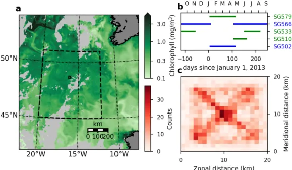
Five Seagliders (gliders) were deployed in a 20 ×20 km region of the northeast Atlantic Ocean over a full year as part of the OSMOSIS project (Figure 3.1a,b) (Thompson et al., 2016; Damerell et al., 2016; Buckingham et al., 2016). Staggered glider deployments ensured that the region was always sampled by at least two gliders, although instrument issues for one glider during November–December 2012 rendered some of the data unusable (Figure 3.1c). Glider data processing, including thermal lag and salinity corrections, is described by Damerell et al. (2016). Glider CTD (conductivity-temperature-depth) measurements were made at approximately 1 m depth intervals. CTDs were calibrated with ship measurements made during deployment and recovery of each glider. A subsequent filter that removed any profile with an average salinity of less than 35.1 PSU or temperature less than 9°C was also found necessary to remove bad dives.

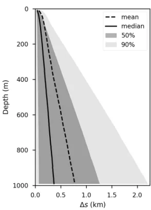
The gliders were piloted in bowtie patterns, with approximately five dives per leg, within the OSMOSIS region (Figure 2.1b). Each ‘V’-shaped dive lasted approximately 5 hours and the horizontal spacing between dives was generally 2–4 km;

each leg of the bowtie pattern lasted approximately one day. The glider location is transmitted before and after each dive, and the horizontal glider position during the dive is linearly interpolated with respect to time between these two points. Location error produced in this interpolation is small (see Appendix). Occasionally the gliders were advected out of the area shown in Figure 3.1c; these data were not used for the following analysis.

Mooring observations

In addition to gliders, nine moorings were arrayed in two concentric quadrilaterals with side lengths of 2–3 and∼13 km around a central mooring (Figure 3.1d). The moorings were instrumented with CTDs and Acoustic Current Meters (ACMs) at 20 to 200 m intervals within the upper 600 m (Figure 2.1e; see Buckingham et al.

(2016) or Yu et al. (2019) for more details). ACMs recorded velocity data at 10 minute intervals and CTDs at 5 minute intervals; for this study CTD data were sub- sampled to ACM temporal resolution. Nine moorings resolve 36 different separation distances, which range from 1.2 to 18.8 km (Figure 2.1e, open circles).

The moorings were subject to currents in the area, and pressure sensors on each CTD

(29)

Figure 2.1: (a) Bathymetry from ETOPO in the northeast Atlantic. OSMOSIS region is shown in the white box at 16.2^◦W, 48.7^◦N. Larger region from the model is shown as the dotted white box. (b) Highlight on the OSMOSIS region, showing a histogram of glider surface locations (colors) and the positions of the nine moorings (x’s). (c) Periods of time in which the gliders were active. (d) Depth placement of the ACMs (x’s) and CTDs (-’s) for each mooring. Dotted horizontal lines denote the depths over which mooring structure functions were calculated. (e) Histogram of structure function pairings from glider measurements at 200, 400, and 800 m depth.

Bins are equally spaced logarithmically. Circle markings at the top axis show the separations between moorings.

(30)

and ACM recorded deviations in depth of up to 150 m. These vertical deviations introduce error into the horizontal distance between moorings; however, in a separate analysis Buckingham et al., 2016 found that the buoyancy applied to the mooring cables restricts their lateral movement and creates an effective pivot point near 600 m depth; stochastic modeling predicted horizontal drifts rarely exceeding 500 m.

High-resolution model

We also analyze a region of the llc4320 model, a high-resolution 1/48° global MIT- gcm simulation. The model is initialized from ECCO2 (Estimating the Circulation

& Climate of the Ocean, Phase II) output (Menemenlis et al., 2008), after which the resolution is increased sequentially to 1/12°, 1/24°, and finally 1/48° (Wang et al., 2018; Torres et al., 2018). The name represents the domain configuration (Latitude- Longitude-polar Cap) and the number of grid cells in the polar cap (4320×4320).

The llc4320 is forced by 6-hourly ERA-Interim atmospheric reanalysis and 16 tidal components. Here we use one year (10 September 2011 to 09 September 2012) of model output from an approximately 120×120 km box centered on the OSMOSIS location (Figure 2.1a, dotted outline) and extending from the surface to 1 km depth, with a horizontal resolution of approximately 1.5 km and 52 vertical levels ranging in thickness from 1 m at the surface to almost 50 meters at 1 km depth. The model timestep is 60 seconds, and data are saved as snapshots every hour. The effective spatial resolution can be estimated as four times the grid spacing, or approximately 6 km.

The llc4320 output has previously been compared with Argo data in the Kuroshio extension, and showed reasonable vertical density stratification and seasonal variability (Rocha et al., 2016b). Globally, Qiu et al. (2018) found consistent surface eddy KE distributions between those inferred from AVISO and llc4320 sea surface height after the latter was coarse-grained to AVISO resolution. Comparisons with submesoscale-permitting observations are limited, but Viglione et al. (2018) found instances of surface instabilities at submesoscales that were temporally and spatially consistent with glider observations in Drake Passage.

Although previous work has validated a number of aspects of this model, care must be taken in making a comparison toin situdata. The model does not assimilate data, and in particular does not reproduce discrete events such as the occurrence of an eddy within a domain at a specific time. While the external forcing is from re-analysis data, the llc4320 output (Sep 2011–Sep 2012) does not match the timeframe of the

(31)

regions (Rocha et al., 2016b; L. Thomas et al., 2016). The site experiences a strong seasonal cycle, which is primarily seen in annual variation of the MLD (Thompson et al., 2016; Damerell et al., 2016; Erickson and Thompson, 2018), calculated from gliders and model output as the depth at which the potential density reaches 0.03 kg m⁻³above the potential density at 10 m (Figure 2.2a) (de Boyer Montégut et al., 2004). During autumn (October–December) the MLD steadily increases, with highly variable wintertime MLDs (January–March) reaching 400 m. These seasonally deep mixed layers lead to the production of Subpolar Mode Water in this region (McCartney and Talley, 1982). The model accurately captures the autumnal increase, wintertime variability (note that only domain-averaged values are shown), and shallow summertime values, but with a deeper mean depth during winter.

Average potential density profiles show a clear seasonality near the surface (Figure 2.2b), with a sharp pycnocline in the summer (green) absent during winter (blue).

The pycnocline is also visible in vertical buoyancy stratification bz ≡ N² of over 10⁻⁴s⁻²below the mixed layer in summer, but without a similar increase at the base of the wintertime mixed layer (Figure 2.2c). The main pycnocline, characterized by N²∼ 10⁻⁵s⁻², is located at about 800 m. We note that the model is lighter than the observations throughout the year, but this does not influence the structure function results below. The model also does not fully capture the strength of the summertime pycnocline (inset to Figure 2.2b).

We treat spice (Π), the component of temperature and salinity that does not contribute to density (Veronis, 1972; Munk, 1981), as a passive tracer. This approximation is valid in the absence of double-diffusive effects, which are small in this region (Damerell et al., 2016). Spice is calculated using the algorithm from McDougall and Krzysik (2015). Time series of spice during the winter–spring transition from

(32)

Figure 2.2: (a) MLD from glider (grey line; black line is filtered through a Gaussian window with standard deviation of 1 day) and model (black dotted line, as an average over the model region marked in Figure 3.1a). For the gliders, the date is in reference to 01 January 2013; the model reference is to 01 January 2012. Summer and winter times are indicated by green and blue shading, respectively. Average potential density (b) and vertical stratificationN² = bz (c) for summer (green) and winter (blue) from glider measurements (solid line), moorings (dashed line), and the model (dotted line). Shading indicates the 50% confidence interval for glider measurements. Inset in panel (b) highlights the upper 100 m of the water column.

Bars in panel (b) represent the mixed layer depth (MLD) of 90% of the measurements for winter (blue) and summer (green) from gliders (SG) and the model (LLC).

(33)

Figure 2.3: Spice along isopycnals for 15 days during April–May from a glider (a) and a single horizontal position in the model (b).

glider measurements show remarkable small-scale features extending to the very bottom of the glider measurements at 1000 m (Figure 2.3a,b). Here we eliminate the heaving effects of internal waves by considering spice along potential density rather than pressure surfaces. These features are consistent over many dives (roughly five per day) and over a range of potential density surfaces. The model also shows high spice variability at depth in coherent subductive events, such as one seen in day 115–118 (panel b; note that the alignment with an observed subductive event is coincidental).

Snapshots of spice at potential densities of 27.03, 27.07, and 27.31 kg m⁻³, corresponding to average depths of 200, 400, and 800 m, respectively, showcase the processes captured by the model (Figure 2.4). A low-spice, mesoscale eddy in the north-west corner of the domain (dashed black boxes) stirs water masses into narrow, elongated filaments. A larger, anticyclonic eddy to the south-east of the domain has a high spice anomaly, and T-S characteristics suggest it is sourced from Mediter- ranean water outflow. A long filament stretches from this eddy into the center of the region studied here. The black boxes in panels e–g represent the size of the

(34)

Figure 2.4: Model snapshots of spice on day 117 (April 28, 2012) for isopycnals 27.03, 27.07, and 27.31 kg m⁻³, corresponding to average depths of 200, 400, and 800 m. Spice is shown as an anomaly from the average value in each panel domain.

Black boxes give the size of OSMOSIS region (solid white box in Figure 3.1a), and the dashed black box is the domain over which the model SFs are calculated (the dashed white box in Figure 2.1a). Figure 2.3b is taken from the center of these boxes.

OSMOSISin situ domain (Figure 3.1b). The high-spice anomaly associated with this filament is strongest at depth. However, although the filament width is narrow compared with the size of the eddy, it is large compared with the OSMOSIS domain and the separations resolved by in situ gliders and moorings. The exceptionally sharp features in the glider data are therefore not captured in the model.

Tidal influences, and especially the M2 tide, are pronounced in this region, as seen in the sharp peak at the M2 frequency in KE, PE, and spice power (Figure 2.5). The sub-inertial component of these variables agrees well between the moorings and the model; however, the model is missing considerable energy in the superinertial range of the spectra. In the mooring data, the superinertial range closely follows the Garrett and Munk (1975) (GM) spectrum for internal waves.

2.4 Structure Functions

Wavenumber spectra are traditionally used to assess tracer variance as a function of scale. However, not all datasets are amenable to spectral decomposition. Structure functions (SFs), defined below, are a useful technique when observations, such as from surface drifters (Balwada et al., 2016) or Argo floats (McCaffrey et al., 2015),

(35)

Figure 2.5: Frequency spectra of KE (a), PE (b), and spice power (c) at 350 m from the model (black) and the moorings (gray). Black dotted lines give the GM spectra, using the formula from Garrett and Munk (1975). Dashed vertical grey lines give the local planetary vorticity (f) and M2 tidal frequencies, and representative slopes of -2 and -3 are shown.

do not follow defined transects.

Thenth-order SF of a scalar tracerθis

Dⁿ_θ(s)=[θ(x) −θ(x+s)]ⁿ, (2.1) where x is a position, s a separation distance, and boldface variables are vectors.

In general x and s can be multi-dimensional, but for this study x represents a latitude/longitude position, s ≡ |s| denotes a horizontal distance and an implied temporal constraint on time differences between measurements (see below), and the overbar is an average over allxin a given time window.

SFs provide information on how variance (or skewness, kurtosis, et cet. forn > 2) changes as a function of separation distance, without requiring that all regions be sampled, as may be the case for power spectra decompositions. The second-order SF is related to the variance spectrumEθ(k)as (Webb, 1964; Babiano et al., 1985)

D²_θ(s)= 2

∫ ∞

0

Eθ(k) [1−cos(k s)]dk. (2.2) AssumingE_θ(k)is represented byak^−λ, for 1 < λ <3 the associated shape ofD²_θ(s) isαs^γ, where (McCaffrey et al., 2015)

γ =λ−1. (2.3)

(36)

In analogy to spectra of KE and PE, we define DK E = 1

2

D_u²+D²_v

and (2.4a)

DPE = D²_b 2bz

, (2.4b)

wherebis buoyancy,u,v are the velocities in the x,ydirection, and the zsubscript denotes partial differentiation in the vertical. Although horizontal velocities from gliders can be estimated using depth-average current calculations and assumptions of thermal wind shear, there is no reliable way to estimate the vertical structure of along-track velocities. We therefore do not attempt a calculation ofD_KEusing glider data.

Applying the SF framework to different types of datasets in a consistent way is challenging due to differences between the different datasets. Due to their ‘V’- shaped dives, gliders sample the same depth at time separations spanning seconds to hours. While multiple gliders were generally in the water at the same time, permitting in theory simultaneous measurements, to achieve the necessary number of measurement pairings at different separations (Figure 2.1e) it was necessary to allow measurement pairings with up to 3 hour temporal separation. For separations of 1 km motions at 10 cm/s and faster are therefore aliased into the results. However, modifying this threshold slightly does not meaningfully change the qualitative results in this paper, and shortening it significantly degrades the number of observations.

For the moorings, we allow only simultaneous (within 5 minutes) measurement pairings, but must contend with vertical movements of moorings through the water column due to internal wave activity. These were recorded by pressure sensors on each CTD and ACM instrument. We only calculate mooring SFs along 6 depths that are well-instrumented (Figure 2.1d, horizontal dotted lines), and only allow measurements that were taken within 10 m of these target depths (using the simultaneous pressure measurements).

For the model, we used the domain represented by the dashed black boxes in Figure 2.4, and only permitted pairings within the same model snapshot. This represented 80×80 pixels, or over 40 million possible pairings. We randomly selected 750 points throughout the domain, for over 500,000 pairings. Random sampling of other 750-point sets did not meaningfully change any of the calculated statistics.

Other details of computing the SFs using the in situ datasets are given in the Appendix.

(37)

Figure 2.6: Structure functions (SFs) for kinetic energy (KE; a), potential energy (PE; b), and spice (Π; c) for winter (see Figure 2.2a) at 350 m from gliders (solid), moorings (dashed), and the model (dotted). Blue lines correspond to the standard SF calculation; grey lines are only using super-inertial frequencies as described in the text. The 90% confidence interval from a bootstrap analysis is given in light shading for the glider results. Confidence intervals for the mooring and model are not shown, but are small compared to those for the gliders. Representative slopes ofs¹ands¹^/²are shown in each panel.

2.5 Results

We construct SFs of KE (D_KE; Equation 2.4a), PE (D_PE; Equation 2.4b), and spice (¹₂D²_Π; Equation 2.1) from the gliders, moorings, and model during winter and summer. The results for winter at 350 m depth are shown in Figure 2.6. Slopes for D_KE and D_PE for in situ data are close to 1, corresponding to a spectral slope of k⁻². The passive tracer SF,D²_Π, is significantly shallower, at a slope of close to 1/2, or k⁻¹^.⁵. SF slopes of KE and PE show good agreement between the model and in situmeasurements at scales of 4–20 km (Figure 2.6a,b). At scales smaller than about 4 km, the in situ measurements from gliders and moorings are both much flatter than the model. Spice SFs are in general much flatter in the observations than the model results, indicating greater spice variance at small scales (as seen in Figures 2.3 and 2.5). At larger scales, the model slope decreases, representing a saturation of variance at scales approaching 100 km. This is consistent with the lack of larger-scale features in this region.

We test the influence of internal wave heaving by calculating SFs along the isopycnal surface most closely aligned to this depth, and do not find a significant difference, indicating that internal waves have only a small imprint on this analysis (not shown).

(38)

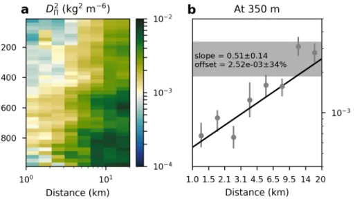
Figure 2.7: (a) Structure function of spice power at all depths from the glider using winter time data. (b) Example of calculating best-fit slopes for a representative SF taken from 350 m depth on panel (a). Black line gives the best fit to the data, and grey horizontal bar shows the range of values of the offset, defined as the variance at 20 km separation.

We decompose the model and mooring measurements into super- and sub-inertial components by filtering out signals at frequencies less than and greater than 16 hours, respectively, corresponding to the local inertial period. The mooring super-inertial SFs are spectrally flat, and can even be dominant over the sub-inertial component for D_KE and D²_Π at scales less than 5 km (sub-inertial results not shown, but are equivalent to the sub-inertial SFs subtracted from the full SF). The model results, in contrast, show little variance associated with super-inertial motions, and the sub- inertial SFs are similar to the full SF at all scales. This is an important result from thisin situdataset, as theoretical and numerical models of stirring in the ocean do not typically account for super-inertial motions (e.g., Smith and Ferrari (2009)).

SFs can be calculated at any depth to provide a full vertical structure of variance in a given property. An example for wintertime spice variance from gliders is shown in Figure 2.7a. This calculation reveals larger spice variance with increasing depth and increasing separation. In particular, the ability to resolve spice variance at scales below 20 km at up to 1 km depth is a major asset of this dataset.

In the range spanning 1–20 km, this information can be well-summarized by a

(39)

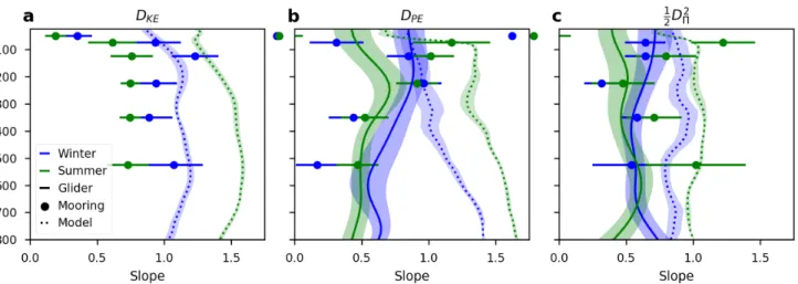
Figure 2.8: Best-fit slopes of KE (a), PE (b), and spice (c) structure functions from gliders (solid), moorings (dots), and model (dotted line) during winter (blue) and summer (green). Shading and error bars show the standard deviation of the fits.

power-law curve

D²_Π = b(s−s₀)^γ, (2.5)

wherebis an ‘offset’ representing the variance at a separation of s₀ = 20 km. We fit the SFs to Equation (2.5) using a Levenberg-Marquardt minimization algorithm (example shown in Figure 2.7b). Weights for thein situ calculations are given as inverse standard deviations, calculated as the spread of the 90% confidence interval divided by 3.29 (i.e., assuming Gaussian distributions). For the gliders, we smooth the final band γ results vertically with a Gaussian window with a standard width of 3 pixels (75 m). For the mooring data, we only calculate the SFs along depth surfaces with sufficient measurements (see Figure 2.1d), corresponding to 50, 75, 125, 225, 350, and 525 m. For fits to modeled data we use only SF calculations for sbetween 4 and 20 km, as this s-domain has relatively uniform slope.

The best-fit slopes (γ) for winter and summer are shown in Figure 2.8. Shading and error-bars give the standard deviation on the fit; however, this is an incomplete description of the full uncertainty. In some instances slopes (and offsets, discussed below) can vary depending on the precise time range chosen for winter and summer, and since we only have one year of data de-convolving seasonal effects with either inter-annual oscillations or chance occurrences in one year, such as an eddy drifting into the region, is not possible. We therefore only comment on those properties that we believe to be robust.

(40)

Thein situslopes forDK E reveal surprisingly little seasonal variance, and are rather constant with depth, at about 0.7 (Figure 2.8a). The model, in contrast, shows a striking seasonality, with slopes increasing dramatically, indicating less variance at small scales, during the summer. ForDPE, the slope varies with depth in the upper 200 m in the summer, being small (greater variance at small scales) near the surface and increasing throughout the summertime pycnocline (Figure 2.8b). During the winter, evidence of a clearly defined mixed layer is muted. For the in situresults there is some evidence that the mixed layer is characterized by a rather uniform slope, which decreases below the average wintertime MLD of about 200 m. The model shows a much clearer transition across the base of the mixed layer base, with a dramatic increase in slope associated with the summertime pycnocline, and a smaller increase starting at the base of the wintertime mixed layer.

The slopes in spice variance are more difficult to interpret, and seasonal differences probably rely more on the presence of eddies and small-scale filaments moving through the region (Figure 2.8c). However, the larger slope (less variance at small scales) in the model vs. thein situmeasurements, at least outside of the mixed layer, does appear to be a robust result.

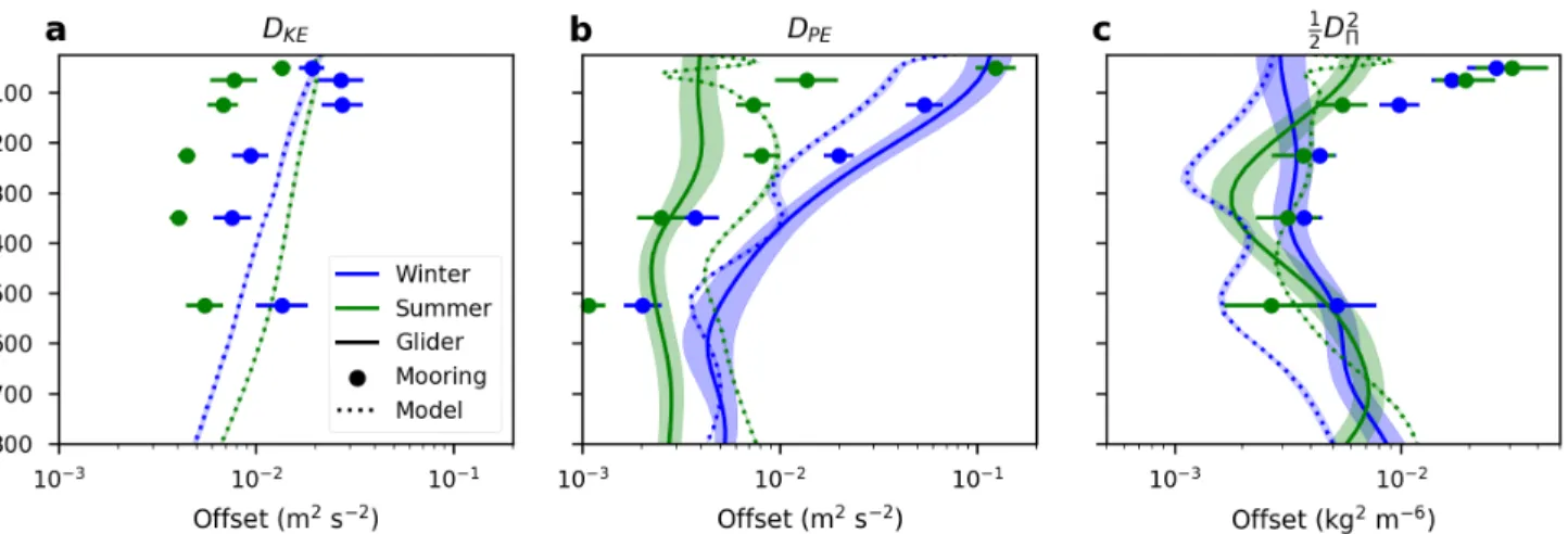
The best-fit offsets (b) are shown in Figure 2.9. In situ DK E offsets show a clear seasonal cycle in the mooring measurements, with higher variance in the winter (Figure 2.9a). Modeled results show a slight increase in summer; however, if values from the beginning of the model run (the previous summer) are added this relationship reverses itself, and we believe this seasonal difference is due to the model not being completely spun up.

The seasonality and vertical dependence in the offsets forDPE(Figure 2.9b) largely follow changes in the vertical stratification bz. It is, however, noteworthy that the model exhibits little seasonality below the base of the wintertime mixed layer, whereas seasonality persists in the in situ measurements down to the seasonal thermocline below 800 m. We believe this to be a signature of vertical mixing below the mixed layer during the winter, as discussed further in the next section.

The offsets in spice power are also shown in Figure 2.9c for completeness; however, as with the changes in slopes we do not believe any of the seasonal or depth variations to be significant.

Calculating best-fit slopes and offsets for time periods throughout the year reveal this seasonal difference between in situand model results more clearly. There are

(41)

Figure 2.9: Best-fit offsets of KE (a), PE (b), and spice (c) structure functions from gliders (solid), moorings (dots), and model (dotted line) during winter (blue) and summer (green). Shading and error bars show the standard deviation of the fits.

small, likely insignificant changes in slopes throughout the year (not shown). The seasonality in offset shows a much larger signal for KE and PE (Figure 2.10). The KE in the model peaks much later, during the spring, than in the mooring results, which have their maximum signal during the winter. For PE, each of the three datasets — gliders, moorings, and model results — peak during in early winter at 50 m and later in winter for the deeper depths. However, the model also has a strong PE signal at 20 km in late spring which is not present in thein situdataset. The cause of this is unclear, but likely related to the dynamics of the spring restratification, which involves small-scale instabilities such as baroclinic mixed layer and symmetric instabilities (Erickson and Thompson, 2018) that will not be fully represented in the model.

2.6 Discussion

Difference between high-resolution model and observations

Because of their utility across a wide range of types of data, SFs are useful to evaluate model fidelity with respect to observations. Here we perform a comparison between in situ and model data output using SFs at 1–20 km resolution. A key difference highlighted in this study is the increased slope of all of the SFs (KE, PE, and spice variance) in the model. The SF values at 20 km, labeled ‘offsets’ or b here, are more comparable, indicating that this increase in slope represents too little variance at small scales. This is an expected characteristic of models, for which variance

(42)

Figure 2.10: Best-fit offsets of KE (a) and PE (b) applied to moving 30-day windows at 50 and 350 m (colors) for gliders (solid), moorings (dashed), and model results (dotted). Data have been smoothed in time.

on scales smaller than about 4-5 model pixels (about 6 km here) is expected to be artificially low, and can also be seen in spectral deconvolutions (e.g., Figure 2.5).

However, we also point to the lack of high-frequency, super-inertial motions in the model as producing this lack of variance at small scales (Figure 2.6). Although the time-step of the model, at 60 seconds, could sufficiently resolve these motions, it is forced with 6-hourly reanalysis winds, which do not input energy at sufficiently high frequencies. Recent work has suggested that models that are subject to surface forcing at super-inertial frequencies develop greater variance at super-interial frequencies, which from Figure 2.6 we suggest will translate into more realistic properties at small spatial scales.

Implications for theoretical models of vertical structure of ocean mixing As reviewed in the Introduction, there exists considerable uncertainty over the expected slopes of passive and active tracers in the ocean interior. In particular, at the surface frontogenesis can cause slopes of k⁻². Far from the surface, active tracers are predicted to have slopes similar to k⁻³, which predicts passive tracers slopes that flatten fromk⁻²to k⁻¹.

Spice SF slopes are near 0.6 and exhibit little seasonality or vertical variability.

Active tracer (K EandPE) slopes estimated fromin situdata are generally between 0.6 and 1. This agrees well with the theoretical relationship between active and passive tracers: for an active tracer SF slope of n the predicted passive tracer SF

Physical processes leading to export of ﬁxed carbon out of the surface ocean

ACKNOWLEDGEMENTS

ABSTRACT

TABLE OF CONTENTS

LIST OF ILLUSTRATIONS

INTRODUCTION