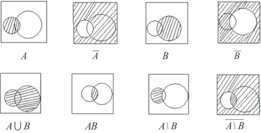
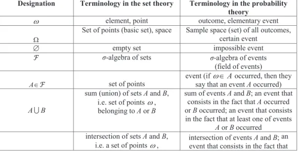
In the textbook, the mathematical foundations of probability theory are presented on the basis of Kolmogorov's axiomatics. The properties of probability are also proven using the axioms of probability theory.
RANDOM EVENTS AND THEIR PROBABILITIES
The probability of a certain event is equal to one
- Elements of combinatorics
The classical definition of probability makes too strict demands on the conditions of the experiment under study. As we saw above, the calculation of the probability of events according to the classical definition reduces to counting the number of elements in some finite quantities, i.e.
Let some finite sets be given
To apply the classical definition of probability, the space of elementary events must be a finite set, and all elementary events must be equally probable (that is, they must have equal probabilities). In connection with the foregoing, it becomes necessary to introduce a definition of probability that would not suffer from the shortcomings of the classical definition and at the same time include a classical definition as a specific case.
- Distribution of balls in boxes
- Tasks for independent work
- Polynomial scheme. The polynomial distribution
What is the probability that the needle will cross one of the parallel planes. Find the probability that the length of the chord will exceed 3r (that is, the length of the side of an equilateral triangle inscribed in a circle).
ІІ
PROBABILITY SPACE
Probability in a measurable space
The construction of a probability space ế:ǡ ࣠ǡ ܲỷ is the main stage in the process of building a mathematical model of the experiment. Therefore, according to axiom P3 (which, under the condition of the theorem, is fulfilled) and determining the sum of the series, we can write: the upper and lower bounds are respectively the events:. Note that an event A in the considered example means that there will be infinitely many events from the sequence of events A1, ,..2. The validity of the above derives from the following chain of relationships:.
An event A is that the point falls exactly in the middle of the segment. If for the set of subsets An:,n 1,2,.. the lower and upper bounds exist and exist. Note that the algebra D D is finite (that is, only a finite number of sets of the form indicated in the definition are entered into it).
The smallest V-algebra (ࣛ), containing ࣛ, is called a Borel -algebra on the number scale, and the elements of the Borel V-algebra are called the Borel sets.
Space (R, β(R)). Distribution function
If for А, Вא ࣠ the probability of their symmetric difference PA'B is 0, then we call such events the equivalent events and denote by ࣛ the class of events thus defined. Show that the thus defined 婩 is a metric on ࣛ and that with this metric ࣛ will be a complete metric space.
The function (1) has the following properties
Thus, by theorem 1, the distribution function F F x( ), defined by (1), corresponds to any probability function P in the space R, ( )E R. The probability measure P constructed from the distribution function F F x( ) is commonly called the Lebesgue-Stiltes probability measure. According to condition F3, the distribution function F F x( ) can have only breakpoints of the first kind.
The fact that the function defined in this way is a distribution function is directly verified. It is clear that the introduced discrete distribution function F x can be represented in the form It turns out that there is a third type of distribution function – this is the so-called simple distribution function.
This type is characterized by the fact that the distribution function F F x( ) is continuous, but the growth point forms a set of Lebesgue measure zero.
The question arises: is it possible to find the types of distribution functions other than the three types defined above? The answer is given by the follo-
Further, each of the remaining segments is again divided into three equal parts, and on the inner segments we define F x as a constant equal to the arithmetic mean between the adjacent, already defined values of F x , etc. At points, that do not belong to such internal segments, we define F x by continuity. It is not difficult to see that the total length of the «internal» segments, on which.
Usually (in particular, in the university courses of probability theory and mathematical statistics), we are dealing only with discrete and absolutely conti-
- Space (R n , β(R n )). Multidimensional distribution function
Let the absolute moment of the k-th order of the distribution function F x be finite: I f. If for a distribution function F x its algebraic (or absolute) moment of the k-th order is finite, i.e. Dk f (Ek f), then for any s kd Dsf (Esf) takes place. D (km), and for ktm the moments of the kth order are not finite. This problem shows that the moments of the distribution function cannot always be finite).
Show that the algebraic moments of the beta distribution with parameters p,q are equal to. Show that the algebraic moments of the chi-square distribution with n degrees of freedom are equal to. We will explain the meaning of probability PB() with the help of the classical definition of probability.
This is the basis for the following definition of the so-called conditional probability.
We saw above that for any event Aא ࣠
- Consider a family with two children. Denote the boy and the girl by letters
- Independence
- Negative binomial distribution. Let’s find the probability that in the sequence of independent Bernoulli trials with the probability of success р the success
- Total probability and Bayes formulas
Kolmogorov, paid special attention to the fundamental nature of the concept of independence in the theory of probability in the thirties of the last century (see [12]) A. If the probability of the product of events A and B is equal to the product of the probabilities of the events A and B, i.e., The independence of the events A1,A2,..,An is equivalent to the independence of the algebra ࣛʏभǡ ࣛʏஜǡ ǥ ǡ ࣛʏ generated by them.
Moreover, according to the probability multiplication formula, a numerator of the formula (25) is equal to , and (according to the total probability formula) the probability of the denominator of (25) is equal to the expression of the denominator of (24). Prove that the probability of placing three balls in one of the boxes is 1/4. Calculate the probability that the balls appeared in the following order: black, white, white, white.
Then what is the probability that the emptiness of the selected matchbox was detected when this (empty) matchbox was first selected.
ІІІ
RANDOM VALUES
The relation
- Discrete random variables
- The event indicator. For the event ܣ א ࣠ we define the indicator of the event А by the relation
- A Bernoulli random variable is a random variable that takes only two values, zero or one, with probabilities
- Poisson random variable. If the distribution law of a nonnegative integer with a random variable is defined by formulas
- Absolutely continuous random variables
In some textbooks (for example, the distribution function is defined as the probability that a random variable falls into a right-open interval. From (7) we find as a special case that the distribution function of a random variable [ is determined by the formula If for a random variable[ its distribution law P[ is determined by relation (7), then such a random variable is called a discrete random variable.
In this case, a random variable that takes a finite number of values is called a simple random variable. Hence for any event ܣ א ࣠ IA1(Z)࣠ we have, therefore (the indicator of event A) IA Z is a random variable. A geometric random variable [ with a parameter p is a random variable that takes non-negative integer values with probabilities.
If for any variable [ there is a non-negative function f x f x [ t0, so the distribution function is written as the integral.
In this text, the integral in (10) will be understood everywhere as an (improper) Riemann integral, in the general case this integral will have to be under-
- Equivalent definitions of a random variable
- Functions of (one) random variable
- The class of extended random variables and the closure of this class with respect to pointwise convergence of this class with respect to pointwise convergence
- Multidimensional random variables and their distributions
- At points of continuity of the distribution density
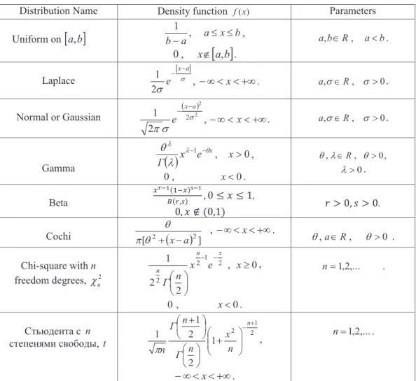
A normal (Gaussian) random variable with parameters (,aV2) is defined as a random variable with a distribution function. Traditionally, the distribution density of a standard normal random variable is usually denoted by M0,1 x or M x (the M x function graph is shown in Figure 2):. By the general definition of a random variable (see Definition 1), to verify that some function [:: oR is a random variable, we must verify that condition (1) holds for any Borel set BE R.
If ln ~[ Na,V2, then the distribution law of the random variable [ is called a lognormal distribution, and the random variable [ itself is called a lognormally distributed (lognormal) random variable. P and the probability measure is called the distribution law of a multidimensional random variable (random vector). ³ , (5') and any function satisfying the property (5') can be the distribution density of some multidimensional random variable.
Hereafter, the so-called multidimensional normal (Gaussian) random variable will be called a multidimensional normal (Gaussian) random variable with parameters.
It turns out that the inverse result is not always valid – from the fact that each component of a random vector is a normal random variable, the normality of
- Independence of random variables
The result obtained in this example – the components of a two-dimensional normal random variable are also normal random variables – remains valid even in the multidimensional case nt3 (this will be shown in Chapter V). It turns out that the converse result is not always valid – from the fact that every component of a random vector is a normal random variable, its normality. Now let us determine the distribution density of a two-dimensional random variable (random vector) [K, as.
For the random variables [1,[2,..,[n to be independent, it is necessary and sufficient that the σ-algebra generated by them ࣠कभǡ ࣠कमǡ ǥ ǡ ࣠क are σ-algebras. Then ࣧ clearly contains the algebra ࣛ of sets consisting of the sum of disjoint intervals of the form I1 a b1, 1@. From the countability of (and thus the continuity of) the probability, it also follows that the system ࣧ is a monotone class (ch. II.
ז From the definition of independence (12) we obtain the following criterion for the independence of (absolutely) continuous random variables.
In the general case, the equality of densities in (13) must be under- stood as an almost sure equality with respect to the n-dimensional Lebegue measure
In order to discrete random variables. were independent random variables, it is necessary and sufficient that for arbitrary xiX, yjY, ..., zkZ,. Obviously, for specific values ,x yi j of discrete random variables [1, [2] there is a rectangle containing only these values. The results of this theorem will usually be used in the form of the statement: “Functions of independent random variables are also independent.
The results of this theorem will usually be used in the form of the statement «The functions of independent random variables are also independent
- Functions of random variables
- Conditional distributions
We ask the following question: by the well-known joint law (joint functions or density) of the distribution of random variables n and given Borel functions. From this we see that the density of the distribution of the ratio [1/[2] is determined by the formula. We show that the density of the distribution of a random variable Fn2 is given by.
After using this formula, find the density distribution of the sum Sn [1 .. [n. b) Find the density of the distribution. Further, from what was said, if [1,[2,..,[n are independent random variables randomly distributed with parameters D, uniformly distributed according to Cauchy's law, then the distribution density of the average. We define a new random vector .. a) the distribution density of the vector K; b) marginal distribution density e) conditional distribution density fK2/K3(x2/y); f) conditional distribution density fK1/K2,K3(x1/y,z).
It is clear that the random variables ξ(1), ξ(2),…,ξ(n) are not independent random variables (the above inequalities apply to them).
MATHEMATICAL EXPECTATION
I. For a simple random variable
We draw attention to the fact that in definition 1 it is not required that the values xii 1,2,..,n taken by the random variable are different, but only that the values xii 1,2,..,n , taken by random variable, be different, but it was only necessary that A A1, 2,..,An partition. Here, by the way, we will explain why the mathematical expectation of a random variable is also called the mean of the random variable.
Here, incidentally, we will explain why the mathematical expectation of a random variable is also called the mean value of a random variable
Consequently, the mathematical expectation M[ , defined above, for n!!1 is indeed an approximation of the mean value of the random variable. For any non-negative random variable [t0, there exists a sequence of simple random variables [n such that 0d[n n[. If a simple random variable [ is written in two ways through finite partitions of the space of elementary events :, i.e.

