Introduction
Contribution of topographically generated submesoscale turbu-
Abstract
The ocean's global overturning circulation regulates the transport and storage of heat, carbon and nutrients. Upwelling over the Southern Ocean's Antarctic Circumpolar Current and in the mixed layer, coupled to water mass modification by surface buoyancy, has been highlighted as a key process in the closure of the overturning circulation.
Southern Ocean overturning pathways
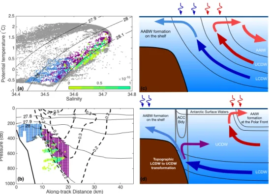
However, isopycnals harboring lower circular deep water (LCDW) do not emerge in regions where the surface buoyancy force is positive, and therefore cannot be converted, through surface transformation, to upper circular deep water (UCDW) ) or in Antarctic intermediate water. AAIW) and participate in the upper branch of the overturning circulation (Naveira Garabato et al., 2014). Instead, it has been suggested that LCDW rises beneath the sea ice and is preferentially entrained in the Antarctic Bottom Water (AABW) and the lower branch of the overturning circulation (Talley, 2013; Ferrari et al., 2014).
Drake Passage glider observations
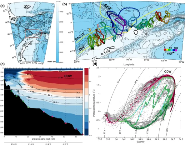
Here we use observations in a region where the southern boundary of the ACC (Bdy) (Orsi et al., 1995) runs along the Antarctic Peninsula continental slope to show that the interplay of strong frontal currents and sloping bathymetry can lead to modification. of LCDW for lighter waters. We focus here on observations collected from the glider deployed west of the Shackleton Fracture Zone (SFZ).
Hydrographic and hydrodynamic information
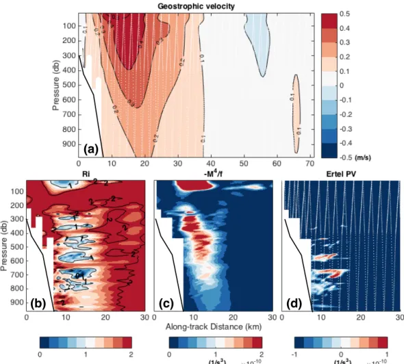
The climatological frontal positions of the Southern ACC Front (SACCF) and the southern boundary of the ACC (Bdy) (Orsi et al., 1995) are shown as yellow contours. Positive PV regions are found on the cyclonic side of the boundary current (from the coast), where.
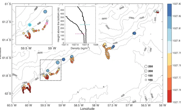
Bottom mixed layers and water mass modification
During flooding, modified water is injected offshore, leading to additional mixing in lighter density classes (Flexas et al., 2015). This process is distinct from the entrainment of LCDW in bottom water plumes that occurs over the continental slope in the subpolar gyres (Orsi et al., 2002).
Appendix A: Methods
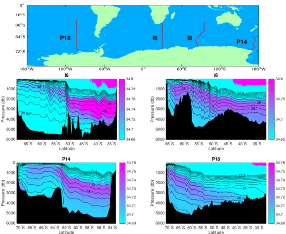
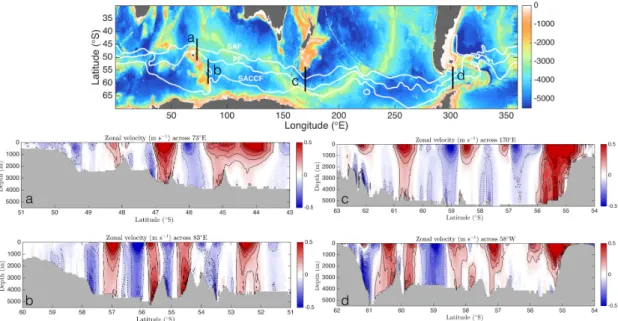
Black contours in the bottom four panels are zonal velocities (eastward, positive, solid lines). Deep reaching fast boundary currents (some with bottom velocity intensification) interacting with the sloping topography can be seen throughout the Southern Ocean over the chosen key topographic features.
Appendix B: Estimates for water mass transformation rates
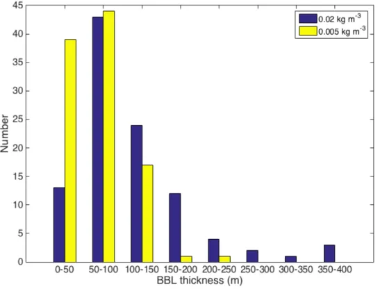
Now we estimate the area of relevant drift surfaces within the BML using the BML thickness of 100 m and a longitudinal distance of 500 km along Southern Drake Passage yielding A = 5× 10⁷ m2. It is important to note that, according to the hypothesis, the excessive (upwelling) diapycnal volume flux along the lower boundary layers should be largely compensated by diapycnal downwelling in the stratified mixed layers globally.
Appendix C: Extrapolation to the circumpolar Southern Ocean using
This means that the bottom stress determines the evolution of the depth-integrated transport in the along-slope direction. Finally, there is a narrow region of divergence of the turbulent buoyancy flux in the pycnocline.
Mixing-driven mean flows and submesoscale eddies over mid-
Abstract
Diapycnic mixing has been found to be slightly enhanced at the bottom over rough topography, particularly over mid-ocean ridge systems that extend for thousands of kilometers in the global ocean. This study investigates the circulation driven by intensified bottom mixing on the flanks of the mid-ocean ridge and within flank canyons, and examines how stratification is maintained to maintain diapycnic transformation.
Introduction
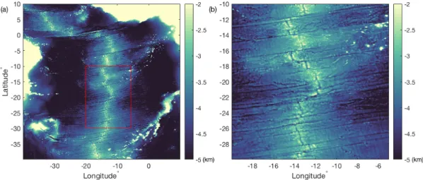
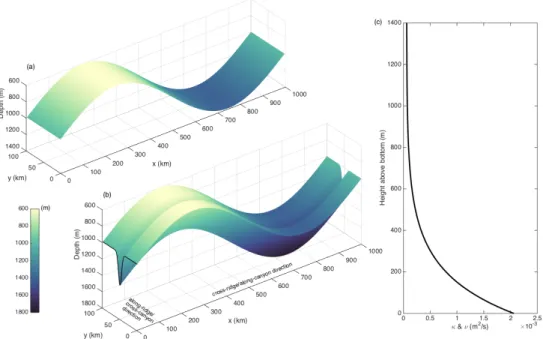
Finally, the contributions to deep-water mass transformation from the various components of the mid-ocean ridge system are discussed. Moreover, across the flanks of the mid-ocean ridges, there are ubiquitous deep canyons that cut across the ridge flank and crest (see Fig. 3.2 for an example in the South Atlantic).
Numerical model configuration
Our focus here is on the subinertial response to under-enhanced mixing over the mid-ocean ridge and within the ridge flank canyons. This is detailed in section 3.4, together with some discussions about the modifications of the induced flow structures compared to those in the planar slope experiments. The prescribed diapycnal mixing acting on the background stratification generates vertical buoyancy that accumulates.
Mean flows and submesoscale baroclinic eddies over mid-ocean ridge
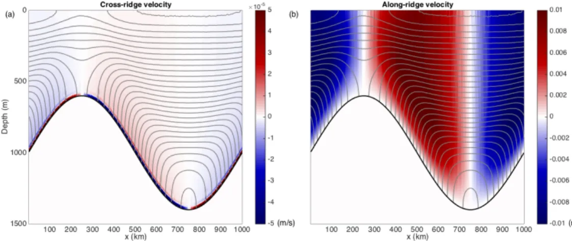
At the same time, the flow reversal in velocity along the slope near the bottom in the one-dimensional system in the two-dimensional simulation disappears (Fig. 3.4c,d). Not only is the structure of the velocity along the slope different, its evolution is much faster in the two-dimensional system. Submesoscale baroclinic vortices (with a vortex size of about 10 km) are found in the mixing layer over the flanks of the ridge (Fig.
Circulation and restratification in ridge flank canyons
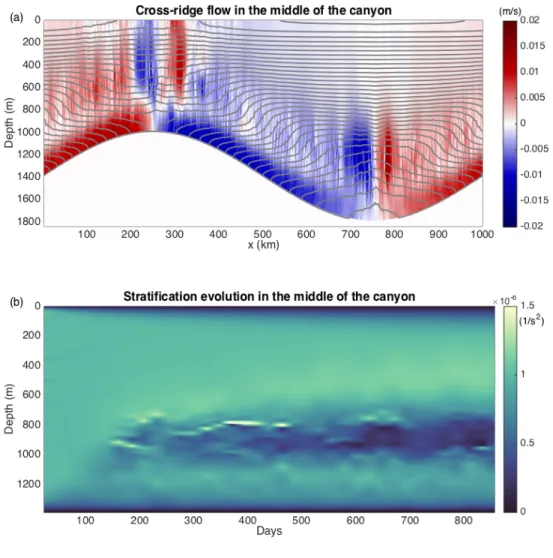
The difference in the size of the cross-slope flow is probably also due to the difference in the canyon width so that the observed canyon (~10km wide) is narrower than the idealized canyon (~20km wide), which is a difference in the blocking effects of the cross-canyon flow (this is explained later). This confirms the role of the canyon walls in the development of the strong up-canyon flow in the three-dimensional simulation (Fig. 3.7). During the simulation, the symmetry in the longslope flowing over the canyon is maintained.

Water-mass transformation in the mid-ocean ridge system
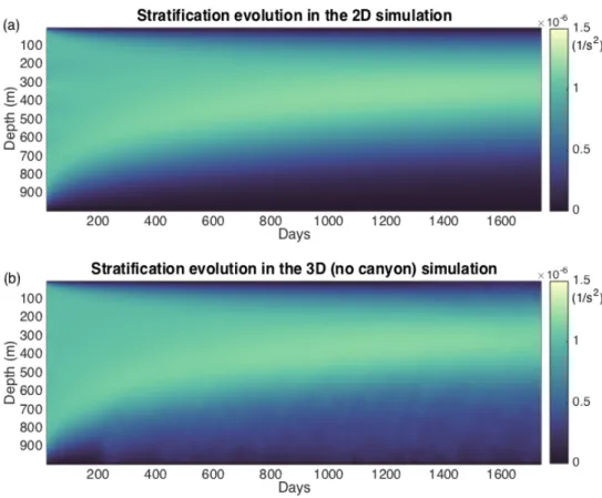
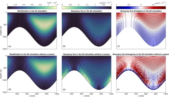
This is best shown in a direct comparison of local stratification, buoyancy flux, and buoyancy flux divergence between two-dimensional and three-dimensional simulations (Figure 3.12). The WMT rates in two-dimensional and three-dimensional cases (without canyon) are shown in the figure. Later in the simulations, the upwelling near the crest of the ridge disappears as the isopycnals bend down towards the ridge and thus the stratification and buoyancy flux become small (Figure 3.12c).
Conclusions
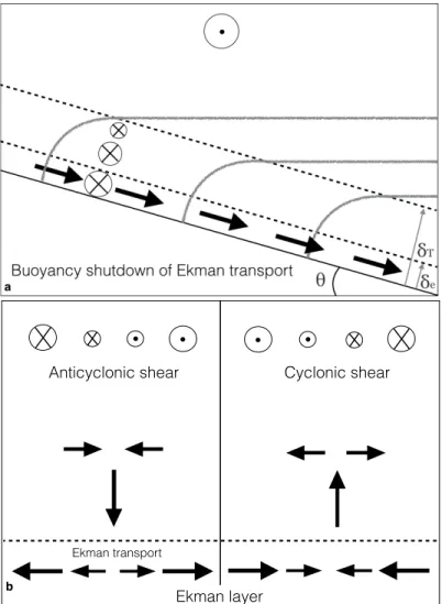
The vertical turbulent buoyancy flux diverges in the lower part of the BBL and opposes the cross-slope advection. The dashed lines represent the upper limits of the Ekman layer (δe) and the thermal boundary layer (δT); gray lines indicate buoyancy contours in the thermal boundary layer. The structure of the velocity and buoyancy fields in the near-inertial regime is similar to the fields shown in fig.
The evolution and arrest of a turbulent stratified oceanic bottom
Abstract
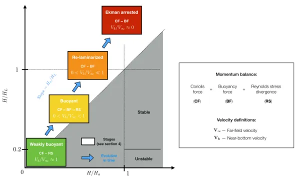
We present two estimates to characterize the state of the BBL based on the mixed layer thickness, Ha and HL. The value of Ha can be combined with the time-evolving mixed layer depth H to form a dimensionless variable H/Ha that provides a prediction of the similarity of BBL development in different turbulent regimes. We conclude that the BBL reaches a re-laminarized state before a stable Ekman-arrested state.
Introduction
When the rotation is combined with the forced mean flow along the slope, the Ekman transport in the cross-slope near the bottom is always smaller than in the case of a flat bottom. Critically, a steady Ekman state has not been observed in the ocean, despite efforts to close the integrated momentum and buoyancy budget in the BBL (Trowbridge and Lentz, 1998). However, the turbulent features associated with the development of the BBL have not been carefully studied in the two approaches presented above.
Theoretical predictions
The near-bottom velocity is the sum of the barotropic mean flow and the opposing thermal wind shear. We show, using LES simulations, that the ratio of H to LS captures the transition of the BBL from. The physical interpretation of the slope Obukhov length Ls is the same as the Obukhov length L.
Numerical methods
The friction velocity u∗ appearing in the non-dimensional parameters does not include layering effects, i.e., scaled and stretched grids are used in the slope-normal direction with finer grid spacing near the upper and lower boundaries . Similar to the SGS model used by Taylor and Ferrari (2010), a constant Smagorinsky model was used in the simulations.
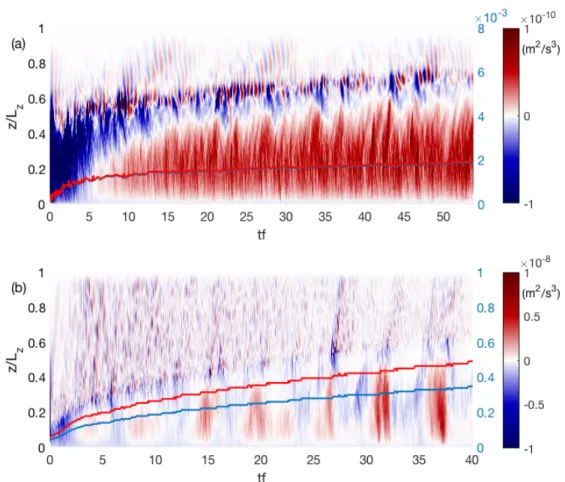
Identification of turbulent regimes from large-eddy simulations
In experiments with larger (initial) values of Bu, the stratification in the pycnocline at the top of the BML is weaker (Fig. 4.7b) during this stage. As Ea and EL become greater than 0.1, the cross-slope velocity profile penetrates deeper into the water column (Fig.. b) The evolution of friction velocityu∗, non-dimensionalized by the initial friction velocity u∗0, as a function of Ea ≡ H/Ha . For cases where the driving force is of leading order, the pycnocline does not sharpen appreciably during the evolution of the BML – the ratio of pycnocline stratification to background stratification is roughly 1 (Fig. 4.7c).
Momentum and buoyancy budgets
AsELTransitions toO(0.1), the Coriolis, buoyancy, and Reynolds stress convergence terms are all of leading order (Fig. 4.16b). The advection of the cross-slope buoyancy occurs mainly in the Ekman layer, which is thinner than the BML (Fig. 4.17a and b). However, the turbulent buoyancy flux converges in the upper part of the BBL, and without a contribution from the cross-slope advection, produces a positive upwelling tendency.
Discussion and conclusions
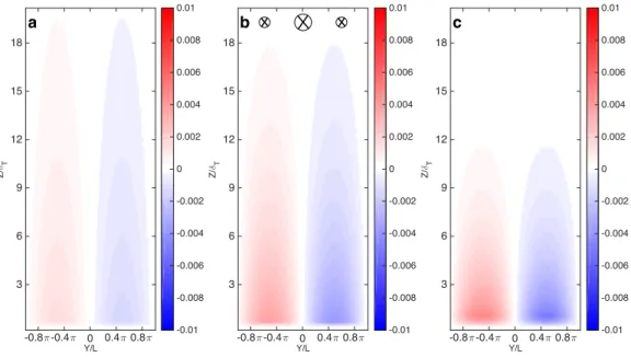
In the following section, we describe numerical simulations of the equations discussed in section 5.4. The PV eddy flux is more sensitive to the amplitude of the topographic slope in the low-frequency regime (Fig. 5.11b). As ω approaches f, resonance in the Ekman layer results in strengthening of the secondary circulation and a peak in the PV flux.
Bottom boundary potential vorticity injection from an oscillating
Abstract
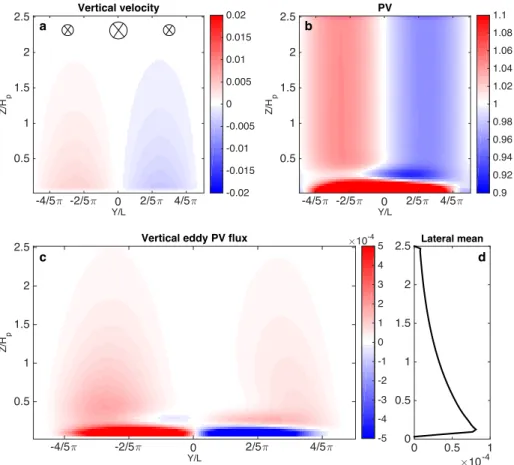
The BBL is responsible for generating a secondary eddy circulation that produces vertical velocities that, together with the PV anomalies of the forced barotropic flow, result in a time-averaged, rectified, vertical eddy PV flux into the ocean interior, the 'PV pump'. In these idealized simulations, the PV anomalies in the BBL secondary contribute to the time-averaged PV current.Numerical results show that the domain-averaged eddy PV current increases nonlinearly with ω with a peak near the inertial frequency, followed by a sharp decline for ω/f > 1.
Introduction
Subsequently, a series of studies have shown that the influence of the boundary layer on the interior can be reduced due to Ekman arrest (MacCready and Rhines, 1991; Trowbridge and Lentz, 1991; Chapman, 2002). Our goal in this study is to understand how a time-dependent mean flow affects Ekman arrest and the general characteristics of the BBL. In this study, we explain how a time-dependent barotropic mean flow reduces the effectiveness of the buoyancy shutdown condition and produces a corrected injection of PV from the BBL into the ocean interior.
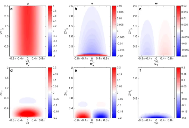
The horizontally sheared and oscillating mean flow model
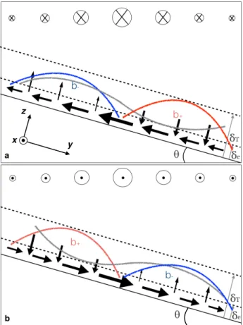
A secondary circulation arises from the convergence and divergence of the Ekman transport corresponding to the lateral sheared mean flow (f > 0). The asymmetry in vertical buoyancy advection causes steeper isopycnal tilting on the anticyclonic flank of the longslope jet. The Ekman layer and the diffuse thermal boundary layer have thicknesses that can be expressed as δe =(2νT )1/2 and δT = (2κT )1/2 respectively, where T is the appropriate characteristic time scale.
Frequency regimes
Thus, in the low-frequency regime, ω/f 1, we assume that the Ekman layer is always fully developed, even though it evolves in time. In the quasi-inertial regime, α is O(1), which mainly affects the Ekman layer as discussed below. Scaling for the thermal boundary layer is not affected by higher frequency oscillations in the near-inertial regime.

Model solutions
Non-linearity in the system arises from interaction between the buoyancy field and the vertical velocity in the thermal boundary layer. At longer times, an asymmetry develops in the vertical extent of the buoyancy anomalies, with positive buoyancy anomalies extending further into the interior. In the Ekman and thermal boundary layers, buoyancy anomalies are generated by advection of the upslope and downslope isopycnals and buoyancy diffusion.
PV dynamics
The vertical eddy PV flux is given by w0q0, where 0 represents a deviation from the spatial (transverse slope and depth) mean value. In the interior, the sign of the horizontal shear is correlated with the sign of the vertical velocity due to the secondary circulation, so that the PV flux is always positive. In the low-frequency regime, the vertical eddy PV flux increases rapidly and nonlinearly with an increase in ω/f (Fig. 5.10, inset).
Conclusions
However, in the near-inertial regime, the buoyancy cut-off effect is already weak and therefore changes in θ have almost no effect on the vertical PV current. In the near-inertial regime, the photovoltage injection is affected by the time-dependent Ekman dynamics. Specifically, the PV eddy current is a nonlinear function of oscillation frequencies with high sensitivity in the low-frequency regime; the.
Appendix: Analytical solutions for the buoyancy shutdown process
Conclusions